Week 3 - Solving second order ODEs

What ODE? (Ordinary Differential Equation)

The ordinary differential equation involves a relation between one real variable which is independent say x and one dependent variable say y and the sum of derivatives y’, y’’, y’’’… with respect to the value of x.

Ordinary differential equations applications in real life are used to calculate the movement or flow of electricity, motion of an object to and fro like a pendulum, to explain thermodynamics concepts. Also, in medical terms, they are used to check the growth of diseases in graphical representation.

Examples

• A simple example is Newton's second law of motion, which leads to the differential equation

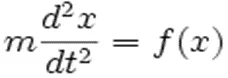
for the motion of a particle of mass m. In general, the force f depends upon the position of the particle x, and thus the unknown variable x appears on both sides of the differential equation, as is indicated in the notation f(x)

• For example, according to the Newton law of cooling, the change in temperature is directly proportional to the difference between the temperature of the hot object or body and the temperature of the atmosphere. Therefore, in terms of the differential equation we can represent it as;

dT/dt ∝ (T – T_a)

Or

dT/dt = k (T – T_a)

Where k is the proportional constant and T is the temperature of the object and Ta is the temperature of the atmosphere.

Objective :

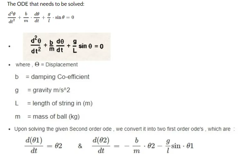
To write a program that solves the Pendulum ODE. This ODE represents the equation of motion of a simple pendulum with damping.

Introduction :

Program :

Function Program :

function [dtheta_dt]=ode_fun(t,theta,b,g,l,m)

theta1=theta(1);
theta2=theta(2);



dtheta1_dt= theta2;                               % ODE 1st
dtheta2_dt=(-g/l)*sin(theta1)-(b/m)*theta2;       % ODE 2nd

dtheta_dt=[dtheta1_dt;dtheta2_dt]  ;              % Both result combine
end

Main Program:

%% ============ plotting pendulum motion w.r.t time =============

clear all
close all
clc

figure (1)
t_span= linspace(0,20,1000);% Time
theta_0= [0,5];             % Inital Condition angular Displacement & Velocity
b=0.05;                     % Damping Coefficient
g=9.81;
l=1;                        % Length of string 'm'
m=0.1;                      % mass of bob in 'kg' 
[t,results]=ode45(@(t,theta) ode_fun(t,theta,b,g,l,m),t_span,theta_0);

a=results(:,1); % Angular Displacement
b=results(:,2); % Angular Velocity

%% Displacement & velocity plot
ax1=subplot(2,1,1);
axis([0 20 -5 5]);
% Now to set the line properties
h1=animatedline('color','r','linewidth',2,'Parent',ax1);
h2=animatedline('color','g','linewidth',2,'Parent',ax1);
yline(0);              % To get Horizontal Line
xlabel('Time')
ylabel('Plot')
title('Plot Angular Displacement & Angular Velocity w.r.t Time')
legend('Displacement','Angular Velocity','Centre ')


%% Pendulum plot
ax2=subplot(2,1,2);
axis([-1.5 1.5 -1.5 0.5]);
axis equal
xline(0);              % To get Verticle Line
hold on
plot(ax2,[-1 1],[0 0],'linewidth',3,'color','b')   % Fixed plot

x0=0;  % Initial X Coordinate of Pendulum string
y0=0;  % Initial Y Coordinate of Pendulum String

x1=l*sin(a);        % 'X' co-ordinates where bob is attached
y1=-l*cos(a);       % 'Y' co-ordinates where bob is attached

l1=line(ax2,[x0 x1(1)],[y0 y1(1)],'linewidth',3,'color','g')   % Pendulum String Plot
p=plot(x1(1), y1(1),'o','markerfacecolor','r','markersize',20) % Pendulum position points
hold off

%% ==================== Animate Plots===================== %%
ct=1;
for j=1:length(t_span)
    
    % add points one at a time to displacement and velocity plot
    addpoints(h1,t(j),a(j));     % Displacement Line
    addpoints(h2,t(j),b(j));     % Velocity Line
    
    % Add points one at a time to pendulum plot
    p.XData=x1(j);         % Bob X-Data of 'p' Variable 
    p.YData=y1(j);         % Bob Y-Data of 'p' Variable
    
    % Animate String
    l1.XData=[x0 x1(j)];    % String X-Data of 'l1' Variable 
    l1.YData=[y0 y1(j)];    % String Y-Data of 'l1' Variable 
    drawnow                 % For creating animation  
    M(ct)=getframe(gcf);
    ct=ct+1;
    
end
    movie(M)
    Videofile= VideoWriter('Second Order ODE of Pendulum')
    open(Videofile)
    writeVideo(Videofile,M)
    close(Videofile)

Outputs :

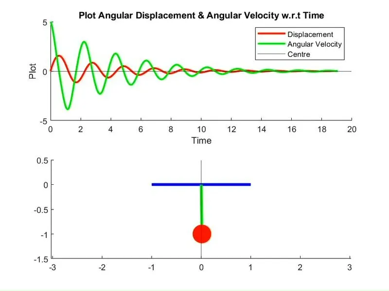
fig. Plot of Angular Displacement and Velocity w.r.t Time

You can watch my video by clicking on Video Link :

https://drive.google.com/file/d/1LHdY_cbMgKJvnV7jTIJKQRl4leSWG66f/view?usp=sharing