Week 4.1 - Genetic Algorithm

AIM:- To optimise the given stalagmite function and find the global maxima of the function.

THEORY:-

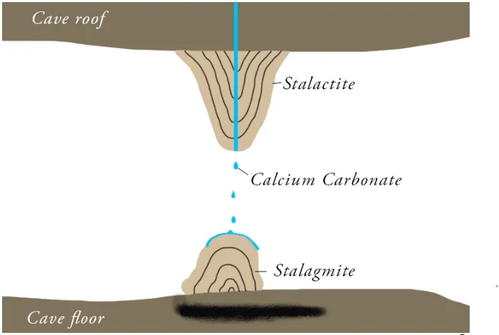
• A stalagmite s a type of rock formation that rises from the floor of a cave due to the accumulation of material deposited on the floor from ceiling drippings. Stalagmites are typically composed of calcium carbonate but may consist of lava, mud, peat, pitch, sand, sinter and amberat (crystallized urine of pack rats ).
• The corresponding formation hanging down from the ceiling of a cave is a stalactits.
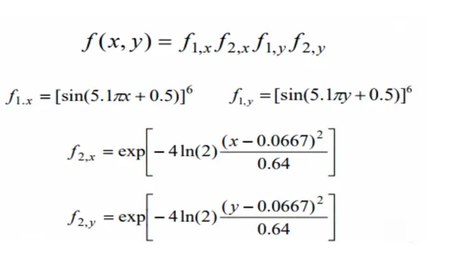
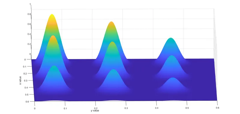
• stalagmite function and stalactite function are mathematical function which represents shapes of the stalagmite and stalactite.

Mathematically we can defind stalagmite function as given below:

Genetic Algorithm(GA):-

• Genetic Algorithm is a search-based optimization technique based on the principles of Genetics and Natural Selection. It is frequently used to find optimal or near-optimal solutions to difficult problems which otherwise would take a lifetime to solve. It is frequently used to solve optimization problems, in research, and in machine learning.
• Genetic Algorithm is a method for solving both constrained and unconstrained optimization problems that is based on natural selection, the process that drives biological evolution. The genetic algorithm repeatedly modifies a population of individual solutions. At each step, the genetic algorithm selects individuals from the current population to be parents and uses them to produce the children for the next generation. Over successive generations, the population "evolves" toward an optimal solution. You can apply the genetic algorithm to solve a variety of optimization problems that are not well suited for standard optimization algorithms, including problems in which the objective function is discontinuous, nondifferentiable, stochastic, or highly nonlinear. The genetic algorithm can address problems of mixed integer programming, where some components are restricted to be integer-valued.

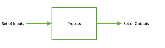
• Optimization is the process of making something better. In any process, we have a set of inputs and a set of outputs
• It uses concepts of evolutionary biology ( Darwin's theory of evolution ) to find the globalminima for optimization problem.

Genetic Algorithm is done in Five steps:

Initial population- The process begins with a set of individuals which is called a Initial Population.

fitness function- The fitness function determines how fit an individual is (the ability of an individual to compete with other individuals). It gives a fitness score to each individual. The probability that an individual will be selected for reproduction is based on its fitness scor.

selection - The idea of selection phase is to select the fittest individuals and let them pass their genes to the next generation.Two pairs of individuals (parents) are selected based on their fitness scores. Individuals with high fitness have more chance to be selected for reproduction.

Crossover - Crossover is the most significant phase in a genetic algorithm. For each pair of parents to be mated, a crossover point is chosen at random from within the genes

mutation - In certain new offspring formed, some of their genes can be subjected to a mutation with a low random probability. This implies that some of the bits in the bit string can be flipped.

Syntax used for GA:-

• x = ga(fun,nvars) | x = ga(fun,nvars) finds a local unconstrained minimum, x, to the objective function, fun. nvars is the dimension (number of design variables) of fun|

• x = ga(fun,nvars,A,b) | x = ga(fun,nvars,A,b) finds a local minimum x to fun, subject to the linear inequalities A*x ≤ b. ga evaluates the matrix product A*x as if x is transposed (A*x') |

• x = ga(fun,nvars,A,b,Aeq,beq) | x = ga(fun,nvars,A,b,Aeq,beq) finds a local minimum x to fun, subject to the linear equalities Aeq*x = beq and A*x ≤ b. (Set A=[] and b=[] if no linear inequalities exist.) ga evaluates the matrix product Aeq*x as if x is transposed (Aeq*x') |

• x = ga(fun,nvars,A,b,Aeq,beq,lb,ub) | x = ga(fun,nvars,A,b,Aeq,beq,lb,ub) defines a set of lower and upper bounds on the design variables, x, so that a solution is found in the range lb ≤ x ≤ ub. (Set Aeq=[] and beq=[] if no linear equalities exist.) |

• x = ga(fun,nvars,A,b,Aeq,beq,lb,ub,nonlcon) | x = ga(fun,nvars,A,b,Aeq,beq,lb,ub,nonlcon) subjects the minimization to the constraints defined in nonlcon. The function nonlcon accepts x and returns vectors C and Ceq, representing the nonlinear inequalities and equalities respectively. ga minimizes the fun such that C(x) ≤ 0 and Ceq(x) = 0. (Set lb=[] and ub=[] if no bounds exist.) |
• x = ga(fun,nvars,A,b,Aeq,beq,lb,ub,nonlcon,options) | x = ga(fun,nvars,A,b,Aeq,beq,lb,ub,nonlcon,options) minimizes with the default optimization parameters replaced by values in options. (Set nonlcon=[] if no nonlinear constraints exist.) Create options using optimoptions. |

• x = ga(fun,nvars,A,b,Aeq,beq,lb,ub,nonlcon,intcon) | x = ga(fun,nvars,A,b,Aeq,beq,lb,ub,nonlcon,intcon) requires that the variables listed in intcon take integer values. |

• x = ga(fun,nvars,A,b,Aeq,beq,lb,ub,nonlcon,intcon,options) | x = ga(fun,nvars,A,b,Aeq,beq,lb,ub,nonlcon,intcon,options) requires that the variables listed in intcon take integer values. |
• x = ga(problem) | x = ga(problem) finds the minimum for problem, a structure described in problem. |

• [x,fval] = ga(___) | [x,fval] = ga(___), for any previous input arguments, also returns fval, the value of the fitness function at x. |

• [x,fval,exitflag,output] = ga(___) | [x,fval,exitflag,output] = ga(___) also returns exitflag, an integer identifying the reason the algorithm terminated, and output, a structure that contains output from each generation and other information about the performance of the algorithm. |

• [x,fval,exitflag,output,population,scores] = ga(___) | [x,fval,exitflag,output,population,scores] = ga(___) also returns a matrix population, whose rows are the final population, and a vector scores, the scores of the final population. |

MATLAB PROGRAM:

• function code:-

function [stalagmite] = stalagmite_func(input_vector)

x = input_vector (1)

y = input_vector (2)

f1_x = (sin(5.1*pi*x +0.5)).^6;

f2_y = (sin(5.1*pi*y +0.5)).^6;

f3_x = exp((-4*0.6931).*(x-0.0667)^2/(0.64));

f4_y = exp((-4*0.6931).*(y-0.0667)^2/(0.64));

stalagmite = (f1_x.*f2_y.*f3_x.*f4_y)
end

• Basic stalagmite program:-

clear all
close all 
clc
% make data for optimization

x = linspace(0,0.6,150);
y = linspace(0,0.6,150);

% 2D GRID

[xx yy] = meshgrid(x, y);

% Stalagmite function

for i = 1:length(xx)
    for j = length(yy)

        input_vector(1) = xx(i,j);
        input_vector(2) = yy(i,j);
        f(i,j) = stalagmite_func(input_vector);
    end
end
surf(xx,yy,f)
shading interp
xlabel('X value')
ylabel('Y value')
[x_output, fval] = ga(@stalagmite_func,2);

Outputs: Workspace

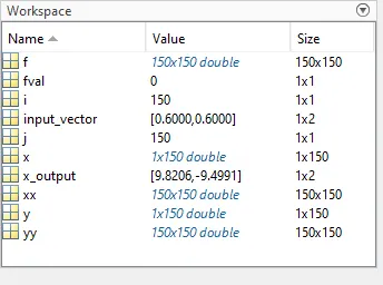
• Main program for optimization:-

clear all
close all 
clc

x = linspace(0,0.6,150);
y = linspace(0,0.6,150);

num_case = 50

% creating 2D grid

[xx, yy] = meshgrid(x,y);

% result of stalagmite function

for i = 1:length(xx)
    for j = 1:length(yy)
        input_vector(1)= xx(i,j);
        input_vector(2) =yy(i,j);
        f(i,j) = stalagmite_func(input_vector);
    end 
end

% case 1 statistical behaviour
tic
for i = 1:num_case
    [inputs,Fopt(i)] = ga(@stalagmite_func,2);
    xopt(i)= inputs(1);
    yopt(i)= inputs(2);
end
study_time_1 = toc;
% ploting
figure(1)
subplot(2,1,1);
hold on
surf(xx, yy, f);
shading interp;
xlabel('x data');
ylabel('y data');
plot3(xopt,yopt,Fopt,'Marker','o','MarkerSize',6,'MarkerFaceColor','y')
title('Unbounded Inputs')
subplot(2,1,2)
plot(Fopt)
xlabel('Iterations')
ylabel('Maximum Function')

% study_2 bounding the values

tic
for i = 1:num_case
    [inputs,Fopt(i)] = ga(@stalagmite_func,2,[],[],[],[],[0;0],[1;1]);
    xopt(i)= inputs(1);
    yopt(i)= inputs(2);
end
study_time_2 = toc;
% ploting
figure(2)
subplot(2,1,1);
hold on
surf(xx, yy, f);
shading interp;
xlabel('x data');
ylabel('y data');
plot3(xopt,yopt,Fopt,'Marker','o','MarkerSize',6,'MarkerFaceColor','r');
title('Bounded Inputs')
subplot(2,1,2)
plot(Fopt)
xlabel('Iterations')
ylabel('Maximum Function')

% study_3 bounding the values and increasing population size.

options = optimoptions('ga');
options = optimoptions(options,'populationsize',300);
tic
for i = 1:num_case
    [inputs,Fopt(i)] = ga(@stalagmite_func,2,[],[],[],[],[0;0],[1;1],[],[],options);
    xopt(i)= inputs(1);
    yopt(i)= inputs(2);
end
study_time_3 = toc;
% ploting
figure(3)
subplot(2,1,1);
hold on
surf(xx, yy, f);
shading interp;
xlabel('x data');
ylabel('y data');
plot3(xopt,yopt,Fopt,'Marker','o','MarkerSize',6,'MarkerFaceColor','g');
title('Bounded Inputs with Increased population size');
subplot(2,1,2)
plot(Fopt)
xlabel('Iterations')
ylabel('Maximum Function')

% end

Final outputs:

CASE1: unbounded inputs

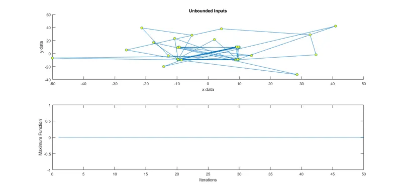
CASE2:Bounded inputs:

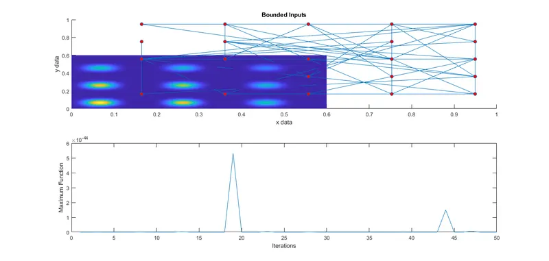
CASE3:Bounded inputs with increased population size: Final workspace data

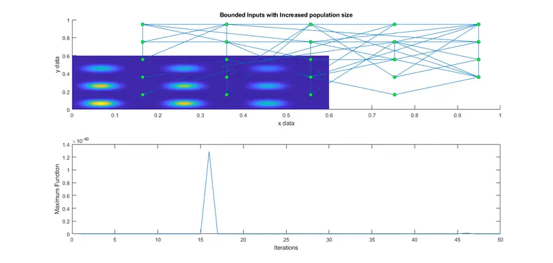
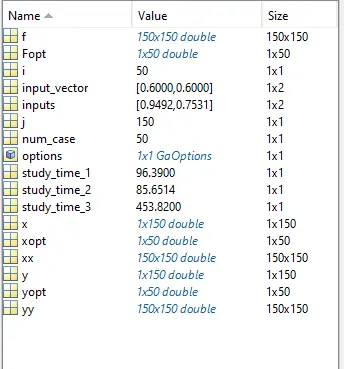
EXPLANTION:-

• Firstly a random array is generated with x & y and by using meshgrid command 2D array is also generated.
• A nested loop is used to assign values from this array into an array named input_vector.
• input_vecror is the input of stalagmite function, and output of stalagmite function is f.
• Tic- Toc command are used to get running time of each case.
• in first case the bounds were not defined and plots were made.
• bounding is given in next case so that the number of solution approaches more accuracy.
• the population is increased in the subsequent cases and plotting is done.
• The iteration were decreased to such a value that the result did not very and the program consumed minimum time to execute.

ERRORS:-

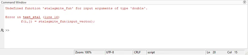
• we defined function by the name 'stalagmite_func' but we call here stalagmite_fun, check and fix it.

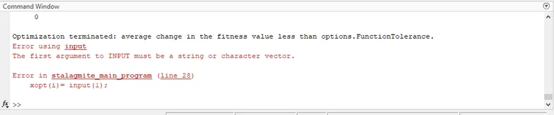
• Here we write 'input' in place of 'inputs' check and fix it.

references:-

• https://in.mathworks.com/help/gads/genetic-algorithm.html
• https://in.mathworks.com/videos/what-is-a-genetic-algorithm-100904.html
• https://in.mathworks.com/help/gads/ga.html