Week 4.1 - Genetic Algorithm
AIM:
To write a programme optimise the stalagmite function and find the the global maxima of the function by using genetic algorithm.
THEORY:
GENETIC ALGORITHM:
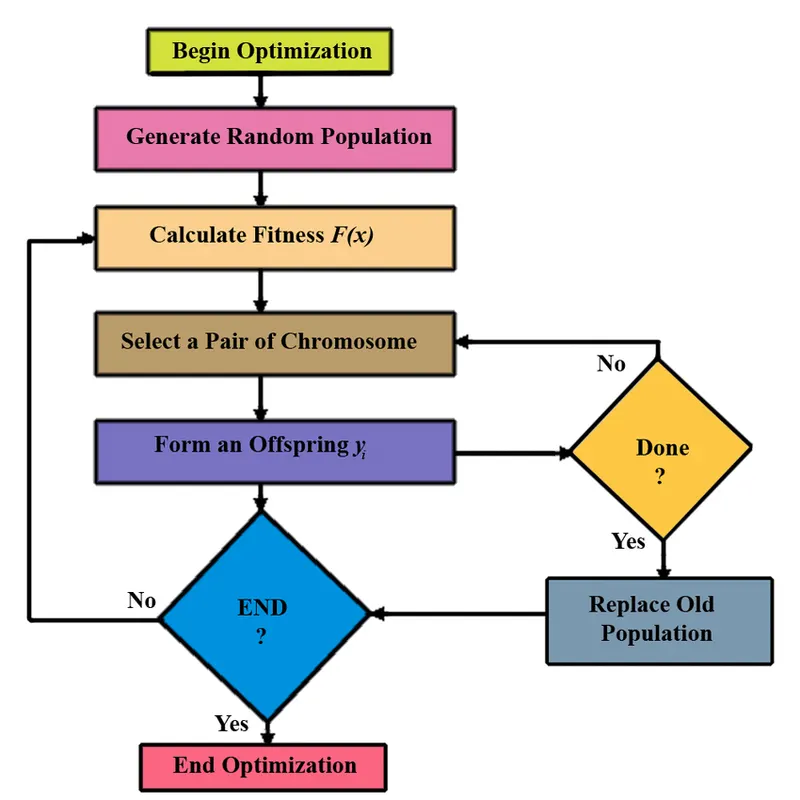
- Genenatic algorithm was based on the principle of darwin's theory of evolution which states that survival of the fittest.
- Here,this algorithm is mainly used to evaluate the solutions of an objective function by considering the random population.Here a fitness function is usually introduction to find the fittest of the solution.This method initially find the parent solution which is termed as the chromosomes,which inturn will undergo a fitness function to find the suitable of solution.Now,set of chromosomesgets mutated by the process of crossover and produce new chromosomes which will be combinations of parent genes.
- Mutation is a process of replacing random genes with another set of random genes.The rate of both crossover and mutation rate value.After several generation the solution value converges to a value which is regarded as the best solution
- Genetic algorithm generally find the local manima which is found to vary each time we run the programme.The consistancy of this can be improved by,Increasing the population size,Assigning the boundedness,Changing the mutation and Crossover rate etc..,
GENERAL SYNTAX OF GENETIC ALGORITHM:
Var_x=ga(@function,nvars,A,b,Aeq,beq,lb,ub,nonlcon,intcon,options).
- @function:The function to be analysed to find the minima
- nvars:This represents the number of the variables to be evaluated
- A,b:This represents the linear inequalities contraints
- Aeq,beq:This represents the linear equalities
- lb,ub:Represents the lower and upper bound values in which the function is to evaluted
- nonlcon:This shows the non linear constraints
- intcon:This represents the integer constraints
- options:These are the option necessary for the algorithm such as population size,crossover function etc to get consistent values.
STOPPING CRITERIA:
In an effort to reduce the lengthy computational time of algorithms, the number of the unique determined schedule is selected as an alternated algorithm stopping criteria condition to identify the trade-off between algorithm stopping criteria and algorithm performance measures.
STALAGMITE FUNCTION (GOVERNING EQUATION):
f(x,y)=f1,xf2,xf1,yf2,y
`f1,x=[sin(5.1pix+0.5)]^6`
`f1,y=[sin(5.1piy+0.5)]^6`
`f2,x=exp[-4ln(2).((x-0.0667)^2/0.64)]`
`f2,y=exp[-4ln(2).((y-0.0667)^2/0.64)]`
STALAGMITE FUNCTION:
function[f]=stalagmite(input_vector);
x=input_vector(1);
y=input_vector(2);

f1=(sin(5.1.*pi.*x+0.5)).^6;
f2=(sin(5.1.*pi.*y+0.5)).^6;
f3=exp(-4*log(2).*(x-0.667).^2/0.64);
f4=exp(-4*log(2).*(y-0.667).^2/0.64);
[f]=-(f1.*f2.*f3.*f4)
end
MAIN CODE:
PROGRAM-1
%MATLAB progrma to find maxima value for stalagmite function GA:
clear all
close all
clc

%defining our search space:
x=linspace(0,0.6,150);
y=linspace(0,0.6,150);
num_cases = 50
%creating 2-dimensional mesh:
[xx yy]=meshgrid(x,y);

%evaluating the stalagmite function:
for i=1:length(xx)
    for j=1:length(yy)
        input_vector(1)=xx(i,j);
        input_vector(2)=yy(i,j);
        f(i,j) = stalagmite(input_vector);
    end
end
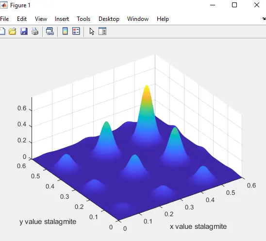
surf(x,y,-f)
xlabel('x value stalagmite')
ylabel('y value stalagmite')
shading interp


[x,fval] = ga(@stalagmite,2);
EXPLANATION:
1.The code is started with the three comands.
clear all-clear the workspace
close all-clear the figure window
clc-clear the command window
2.We define the value of x and y using the linspace().
3.A meshgrid [xx yy] is created using x and y matrix.
4.Then we evaluate the stalagmite function running a for-loop and here we call the stalagmite function.
5.plot the stalagmite function in as a 3D surface.
study of genetic algorithm for the random sampling:
- we run to find the maxima value by running the ga() for 50 times.
- Also we calculate the running time.
- Then we plot the stalagmite function along the maximum values which is we have got from multiple iterations,also we plot function maxima vs iteraction on the same figure.
6.Tic and Toc :Tic works with the toc function to measure the elapsed time.The 'Tic' function records the current function and the 'Toc' function uses to record value to calculate the elapsed.
PROGRAM-2
%case 1:finding maxima without giving any constraints or unbounded value
clear all
close all
clc

%defining our search space:
x=linspace(0,0.6,150);
y=linspace(0,0.6,150);

%creating 2-dimensional mesh:
[xx yy]=meshgrid(x,y);

%evaluating the stalagmite function:
for i=1:length(xx)
    for j=1:length(yy)
        input_vector(1)=xx(i,j);
        input_vector(2)=yy(i,j);
        f(i,j) = stalagmite(input_vector);
    end
end
surf(x,y,-f)
xlabel('x value stalagmite')
ylabel('y value stalagmite')
shading interp

tic
%statical behaviour without bounds:
num_cases = 50
for k=1:num_cases
    [inputs,fopt(k)]= ga(@stalagmite,2);
    xopt(k)=inputs(1);
    yopt(k)=inputs(2);
end
study_time1=toc
figure(1)
subplot(2,1,1)
hold on
surfc(xx,yy,-f)
shading interp
plot3(xopt,yopt,-fopt,'marker','o','MarkerSize',5,'MarkerFaceColor','r')
title('unbounded inputs')
subplot(2,1,2)
plot(-fopt)
xlabel('iterations')
ylabel('function minimize')
EXPLANATION:
Study of genetic algorithm without any constraints or boundedness
- Now here we compute the maxima by using genetic algorithm.
- The syntax of GA include calling the function whose maxima is to be found and the no.of.variables,here begin the case one we do not define the popoulation nor the bounds.
- Since,GA return to maxima value we multiple the results of stalagmite function with a negative sign.
- So the GA return to the maximum value with the negative sign,thus the point of incident of maximum value and the value itself is also stored on to an array.
- The results of stalagmite function is popltted as a 3-Dimensional array and the maxima along with their point of incident is plotted.
PROGRAM-3
%case 2:finding maxima with giving constraints and bounded values
clear all
close all
clc

%defining our search space:
x=linspace(0,0.6,150);
y=linspace(0,0.6,150);

%creating 2-dimensional mesh:
[xx yy]=meshgrid(x,y);

%evaluating the stalagmite function:
for i=1:length(xx)
    for j=1:length(yy)
        input_vector(1)=xx(i,j);
        input_vector(2)=yy(i,j);
        f(i,j) = stalagmite(input_vector);
    end
end
surf(x,y,-f)
xlabel('x value stalagmite')
ylabel('y value stalagmite')
shading interp

tic
%statical behaviour with upper and lower bounds:
num_cases = 50
for k=1:num_cases
    [inputs,fopt(k)]= ga(@stalagmite,2,[],[],[],[],[0,0],[0.6,0.6]);
    xopt(k)=inputs(1);
    yopt(k)=inputs(2);
end
study_time1=toc
figure(2)
subplot(2,1,1)
hold on
surfc(xx,yy,-f)
shading interp
plot3(xopt,yopt,-fopt,'marker','o','MarkerSize',5,'MarkerFaceColor','r')
title('bounded inputs')
subplot(2,1,2)
plot(-fopt)
xlabel('iterations')
ylabel('function minimize')
EXPLANATION:
- Here in the case two we include the bounds which is describes the domain in which the GA has to compuate the maxima.
- The bounds were defined as 0-0.6 for both x and y.The syntax for which is shown below
- Introducing the domain helps to eliminate the unwanted population which will be included to compute the maxima.
- Here also we plot the same compponent as in case 1.
PROGRAM-4
%case 3: Increasing the GA iterations
clear all
close all
clc

%defining our search space:
x=linspace(0,0.6,150);
y=linspace(0,0.6,150);

%creating 2-dimensional mesh:
[xx yy]=meshgrid(x,y);

%evaluating the stalagmite function:
for i=1:length(xx)
    for j=1:length(yy)
        input_vector(1)=xx(i,j);
        input_vector(2)=yy(i,j);
        f(i,j) = stalagmite(input_vector);
    end
end
surf(x,y,-f)
xlabel('x value stalagmite')
ylabel('y value stalagmite')
shading interp

%statical increasing number of iterations
options = optimoptions('ga')
options = optimoptions(options,'populationsize',170)

tic
num_cases = 50
for k=1:num_cases
    [inputs,fopt(k)]= ga(@stalagmite,2,[],[],[],[],[0,0],[0.6,0.6],[],[],options);
    xopt(k)=inputs(1);
    yopt(k)=inputs(2);
end
study_time3=toc
figure(3)
subplot(2,1,1)
hold on
surfc(xx,yy,-f)
shading interp
plot3(xopt,yopt,-fopt,'marker','o','MarkerSize',5,'MarkerFaceColor','r')
title('optimization')
subplot(2,1,2)
plot(-fopt)
xlabel('iterations')
ylabel('function minimize')
EXPLANATION:
- Here the case two we include the bounds as in case 2,also we define the population size.
- The population size were defined as 250.The syntax for which is shown below
- Defining the population size helps to include more of the value from the bounds and hence this helps to include more value.
- Increasing the population size helps to compute for finding the minimum value over the large population which in turn will show approximate the global maxima value when compared to the previous cases.
- The plots are done as same in the previous cases.
RESULTS:
CASE 1: No bounds and population size
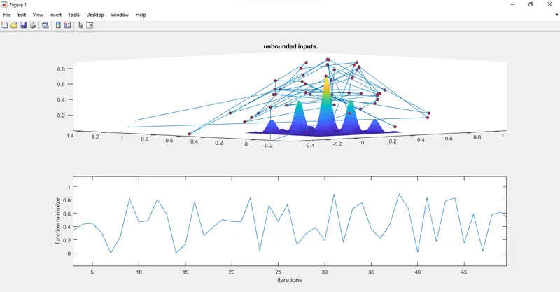
- From the figure, it can be easily interpretted that the maxima at each iteration is found to be scattered all over the plot which is depicts that the found to be maxima rather than a global one.
- This in turn can be cleared depicted from the graph of maxima stalagmite v/s iteration that the maxima just varies randomly over iterations thus make the function less consistant.
CASE 2: Assigning the bounds
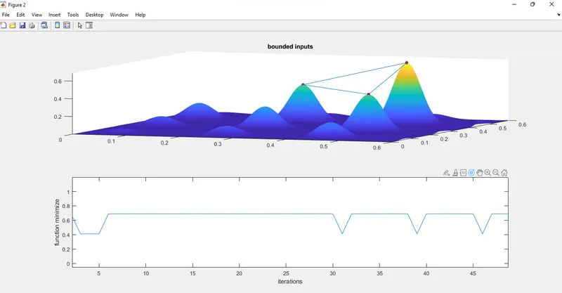
- It shows that the variation of maxima with iteration has consider reduced with respect to case 1.
- This is clearly depicted in the graph of maxima stalagmite v/s iteration where the maxima lies in between (0.4 and 0.7).
- Thus almost value equal to 0.6 is shown which is the value of maxima is converging.
CASE 3: Assigning the bounds and population size
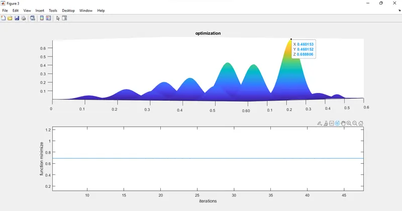
- At this point,defining the population size the ga really considers a large no.of.population to compute the maxima.
- Thus increasing the population size and the population size and by defining the bound the ga gets the clear picture of the domain and this will able to compuate maxima.
- Thus from graph of maxima stalagmite v/s iteration, the variation of the maxima value with the 100 iteration is almost a constant value (considerably small variation which could be negelected) thus on defining the bound and population size a constant value of maxima is found.
- This maxima could be concluded as a global maxima.
LINKS:
General algorithm:https://en.wikipedia.org/wiki/Genetic_algorithm
Stalagmite:https://en.wikipedia.org/wiki/Stalagmite
CONCLUSION:
Hence, the global maxima value is obtained x=0.460159 and y=0.46015 and optimum value is approximately 0.7.