Project 2 - Rankine cycle Simulator

AIM:

Creation of Rankine cycle simulator from given from given input and reading the data from standard thermodynamics library of steam table.

OBJECTIVES:

• Create a rankine cycle simulator using Matlab.
• Your code should be calculate the state points of the rankine cycle based on user inputs.
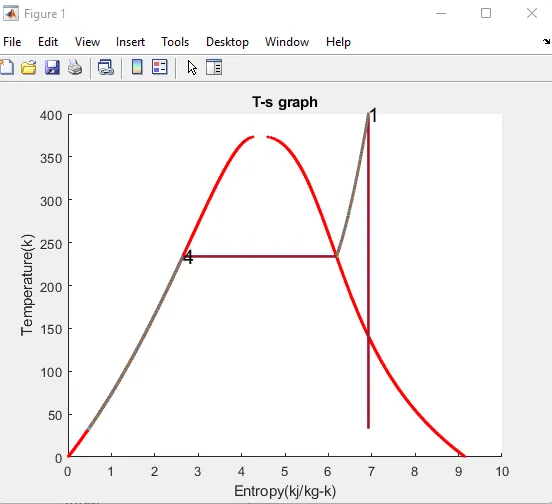
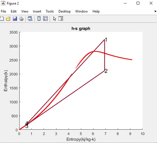
• Then,plot the corresponding T-s and h-s plot for the given set of inputs.Tittle and axis labels are must, while legends could be used if necessary.

INTRODUCTION:

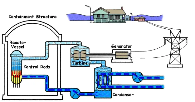
• The Rankine cycle or Rankine vapour cycle is the process of widely open used for power plants such as coal fired power plants such as coal fired power plants or nuclear reactors. In this mechanism, a fuel is used to produced heat within the boiler.
• Converting water into steam which then expands through a turbine producing useful work.This process was developed in 1859 by scottish engineer william J.M Rankine.
• This is a thermodynamics cycle which converts into mechanical energy into electricity, by electrical generation.

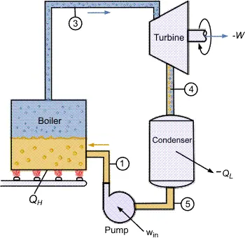
This steps in the rankine cycle as shown in below figure:

1.PUMP:

Compression of the fluid to high pressure using the pump(this takes work).

2.BOILER:

The compressed fluid is heated to the final temperature (which at boiling point).Therefore, a phase change occurs from liquid to vapour.

3.TURBINE:

Expansion of the vapour in the turbine.

4.CONDENSOR:

Condensation of the vapour in the condenser (wherre the waste heat goes to the final heat )sink the atmosphere or a large body of water(ex.lake or river ).

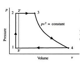
Corresponding steps in the P-V diagram:

• The efficiency of the rankine cycle is limited by the high heat of vapourization by the fluid.The fluid must be recycled through and reused constantly. Thererfore, water is the most practical fluid for this cycle.
• This not why many power plants are located near a body of water that for the waste heat.
• As the water condenses in the condenser,waste heat is given off in the form of water vapour which can be seeen boiling from a plant so they have the cooling towers.
• This waste heat is necessary in any thermodynamics cycle.Due, to this condensation step, the pressure at the outlet is lowered.This means the pump requried less work to compress the water resulting in higher overall efficiencies.

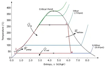
THE FOUR PROCESS IN THE RANKINE CYCLE:

1. PROCESS 1-2 [Isentropic compression]
2. PROCESS 2-3 [Constant pressure heat addition in boiler]
3. PROCESS 3-4 [Isentropic expansion]
4. PROCESS 4-1 [Constant pressure heat rejection in condenser]

GOVERNING EQUATIONS:

In general, the efficiency of a simple rankine cycle can be written as,

`eta_(thermal)= ((W_(thermal)-W)/(Q_(In))) approx (W_(turb))/(Q_(In))`

Each of the next four equation is derived from energy and mass balance sheet for a constant volume. `eta_(thermal)` defines the thermodynamics efficiency of the cycle as the ratio of net power output to heat input.AS per the work requried by the pump is often around 1% of the turbine work output,it can be simplified`

`Q_(In)/m=h3-h2,`

`Q_(out)/m=h4-h1,`

`W_(pump)/m=h2-h1,`

`W_(TURBINE)/m=h3-h4,`

When dealing with the efficiencies of the turbines and pumps, an adjustments to the work terms must be made:

`W_(pump)/m =h2-h1 approx (v1 triangle_(p))/ eta_(pump) = (v1(p2-p1))/eta_(pump),`

`W_(TURBINE)/m= h3-h4 approx (h3-h4) eta_(TURBINE).`

Required Inputs:

Turbine Inlet temperature = 400° C

Turbine Inlet Pressure = 30 bars

Turbine Outlet Pressure = 0.05 bars = Condenser Inlet Pressure

CODE PROGRAM:

% A program to simulate Rankine cycle
clear all
close all
clc

%% Displaying the  process in the command window
disp('process in rankine cycle')
fprintf('\n')
disp('process 1-2: isentropic compression')
disp('process 2-3: constant pressure heat addition')
disp('process 3-4: isentropic expansion')
disp('process 4-1: constant pressure heat rejection')

%% Initialization for variables and parameters
fprintf('\n\n')
t=linspace(0,374,500);
P1=input('Enter the pressure at turbine inlet (bar): ');
T1=input('Enter the temperature at turbine inlet (k): ');
P2=input('Enter the pressure at condenser(bar): ');
fprintf('\n\n')
%% Assign the values of p,h,T,s for each state using the 'Xsteam' library
% At state 1
h1=XSteam('h_PT',P1,T1);
s1=XSteam('s_PT',P1,T1);
hl1=XSteam('hL_P',P1);
hg1=XSteam('hV_P',P1);
sl1=XSteam('sL_P',P1);
sg1=XSteam('sV_P',P1);
Tsat1=XSteam('Tsat_P',P1);

%% At state point 2
s2=s1;
sl2=XSteam('sL_P',P2);
sg2=XSteam('sV_P',P2);
x=(s2-sl2)/(sg2-sl2);
hl2=XSteam('hL_P',P2);
hg2=XSteam('hV_P',P2);
h2=hl2+x*(hg2-hl2);
T2=XSteam('T_ph',P2,h2);
Tsat2=XSteam('Tsat_P',P2);

%% At state point 3 
h3=hl2;
s3=sl2;
P3=P2;
T3=T2;

%% At point 4
s4=s3;
P4=P1;
h4=XSteam('h_ps',P4,s4);
T4=XSteam('T_ps',P4,s4);

%% Plotting T-s Graph
figure(1),clf
hold on

%saturation curve
for i = 1:length(t)
    plot(XSteam('sL_T',t(i)),t(i),'r.')
    plot(XSteam('sV_T',t(i)),t(i),'r.')
end

%% Cycle
plot([s1 s2],[T1 T2],'LineWidth',2)
text(s1,T1,'1','FontSize',15)

if x>1
    T3=Tsat2;
    plot([s2 sg2 s3 s4],[T2 Tsat2 T3 T4],'LineWidth',2)
    T2=Tsat2;
    text(s2,T2,'2','FontSize',15)
    text(s3,T3,'3','FontSize',15)
end

n= linspace(T1,T2,1000);
for i=1:length(n)
    plot(XSteam('s_pT',P1,n(i)),n(i),'.','LineWidth',2)
end

plot([sl1 sg1],[Tsat1 Tsat1],'LineWidth',2)
text(sl1,Tsat1,'4','FontSize',15)
xlabel('Entropy(kj/kg-k)')
ylabel('Temperature(k)')
title('T-s graph')

%% For h-s graph
figure(2),clf
hold on

%% saturation currve
for i=1:length(t)
    plot(XSteam('sL_T',t(i)),XSteam('hL_T',t(i)),'r.')
    plot(XSteam('sV_T',t(i)),XSteam('hV_T',t(i)),'r.')
end

%% cycle
plot([s1 s2 s3 s4 s1],[h1 h2 h3 h4 h1],'LineWidth',2)
text(s1,h1,'1','FontSize',15)
text(s2,h2,'2','FontSize',15)
text(s3,h3,'3','FontSize',15)
text(s4,h4+90,'4','FontSize',15)
xlabel('Entropy(kj/kg-k)')
ylabel('Enthalpy(k)')
title('h-s graph')

%% Calculation
%Workdone by turbine
WT=h1-h2;

%Workdone by pump
WP=h4-h3;

%net workdone
Wnet=WT-WP;

%Thermal efficiency
eff=(1-((h2-h3)/(h1-h4)))*100;

%Back Work Ratio
BWR=WP/WT;

%specific steam conductivity
SSC = 3600/WT;

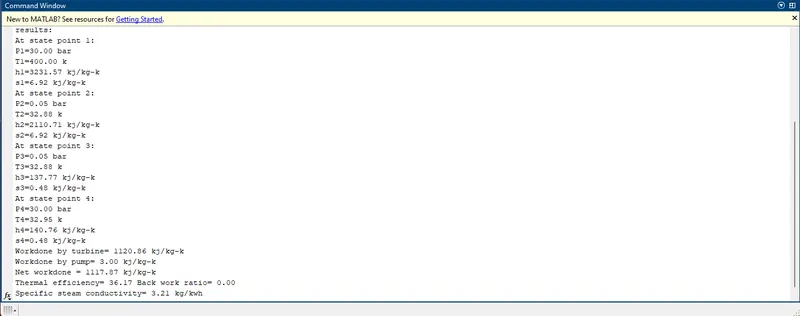
%% display results in command window

disp('results: ')
disp('At state point 1: ')
fprintf('P1=%.2f bar \n',P1)
fprintf('T1=%.2f k \n',T1)
fprintf('h1=%.2f kj/kg-k \n',h1)
fprintf('s1=%.2f kj/kg-k \n',s1)

disp('At state point 2: ')
fprintf('P2=%.2f bar \n',P2)
fprintf('T2=%.2f k \n',T2)
fprintf('h2=%.2f kj/kg-k \n',h2)
fprintf('s2=%.2f kj/kg-k \n',s2)

disp('At state point 3: ')
fprintf('P3=%.2f bar \n',P3)
fprintf('T3=%.2f k \n',T3)
fprintf('h3=%.2f kj/kg-k \n',h3)
fprintf('s3=%.2f kj/kg-k \n',s3)

disp('At state point 4: ')
fprintf('P4=%.2f bar \n',P4)
fprintf('T4=%.2f k \n',T4)
fprintf('h4=%.2f kj/kg-k \n',h4)
fprintf('s4=%.2f kj/kg-k \n',s4)

fprintf('Workdone by turbine= %.2f kj/kg-k \n',WT)
fprintf('Workdone by pump= %.2f kj/kg-k \n',WP)
fprintf('Net workdone = %.2f kj/kg-k \n',Wnet)
fprintf('Thermal efficiency= %.2f % \n',eff)
fprintf('Back work ratio= %.2f \n',BWR)
fprintf('Specific steam conductivity= %.2f kg/kwh \n',SSC)

CODE EXPLANATION:

1. The creationof the rankine cycle simulator starts with some inputs value which are requried to calculate the other state point in cycle eventually.

2. The rankine cycle process is displayed in the command window and then inputs are entered which are inlet pressure for the turbine, temperature at turbine inlet and pressure at condenser.

3. Then we are using the Xsteam function file for reading state point.Frist, we get thee value of enthalpy and entropy at point 1 from the Xsteam file function.

4. As process from 1-2 is isentropic compression the entropy at point 1 is equal to point 2. The term '(s_PT,P1,T1)' refers to the entropy at pressure and temperature point 1.

5. The term 'sg' and 'sf' are referred to saturated vapour entropy respectively.This value is used to calculate other function according to mathematical relations.

6. Similarly, other points are taken from Xsteam function file which is necessary to calculate other parameters. After that workdone in turbine and pump are calculated for further getting the network done Ranklne cycle.

7.After calculating the network done the efficiency of the rankine cycle is calculated along with specific steam consumption which is steam consumed by a locomotion cylinders per unit of output of workdone.

8. Then, temperature at each point of cycle is calculated using input taken from start of the program and data taken from Xsteam file. For given the temperature range from lower to higher enetropy points are calculated to created the T-s plots. Similarly, another for loop is used to create the saturation curve for each plot.

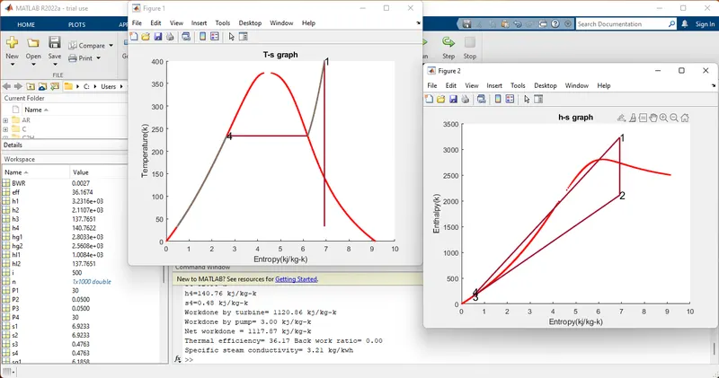
9. Then, plotting is done respectively for T-s and H-s graph in rankine cycle and each state point value has been put in command window.

OUTPUTS:

1.T-s PLOT:

2.H-s PLOT:

3.COMMAND WINDOW:

4. OVERALL OUTPUT SCREENSHOT:

REFERANCE:

https://energyeducation.ca/encyclopedia/Rankine_cycle

https://en.wikipedia.org/wiki/Rankine_cycle

ERROR OCCURED:

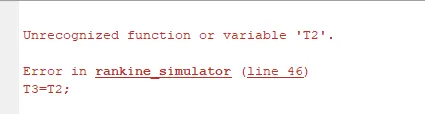
It's about i used lower case t2 instead of T2.so, i endup with this error.Because,matlab is also case-sensitive.

RANKINE CYCLE CALCULATIONS REFERANCE:

Engineering thermodynamics Textbook formulas and calculations.

GOOGLE DRIVE LINK:

https://drive.google.com/drive/folders/1wKCO1FSHWrcvy6St0pnA_-2CugEIegxs

CONCLUSION:

Finally, complete the program for Rankine cycle using matlab and the graph for T-s and h-s were plotted and which, we have taken the data from Xsteam function file.