Project 1 - Parsing NASA thermodynamic data

AIM:

To write a program in MATLAB for parsing NASA thermodynamics data.

OBJECTIVIES:

1. To write a function that extracts the 14 co-efficients and calculates the enthalpy, entropy and specific heat for all the species in the data file.
2. To calculate the molecular weight of each species and display it in the command window.
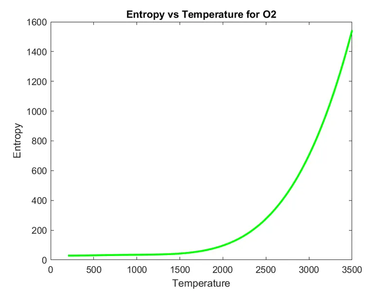
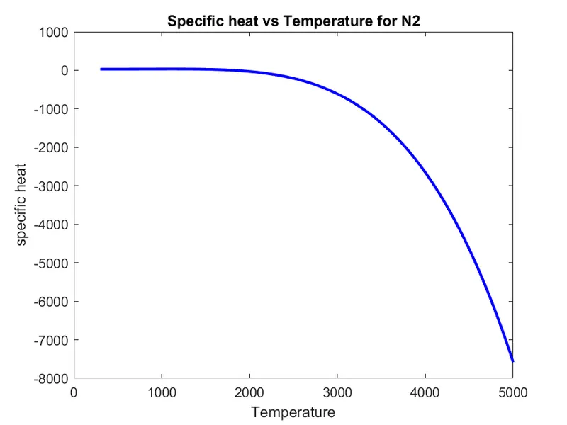
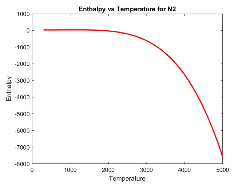
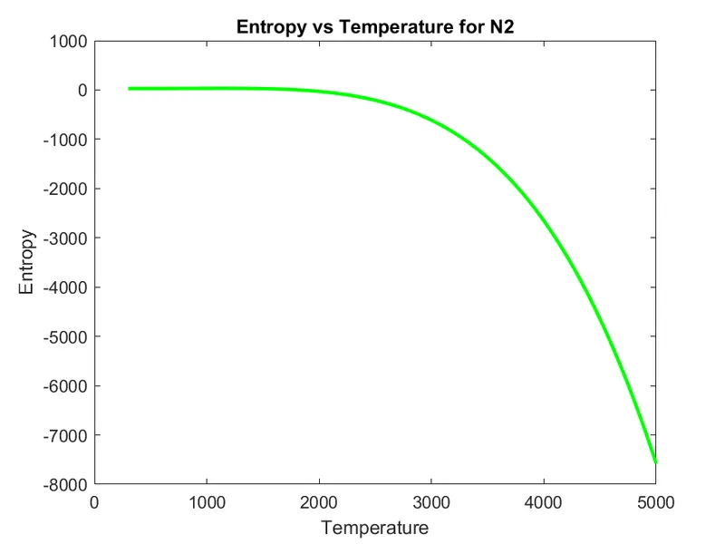
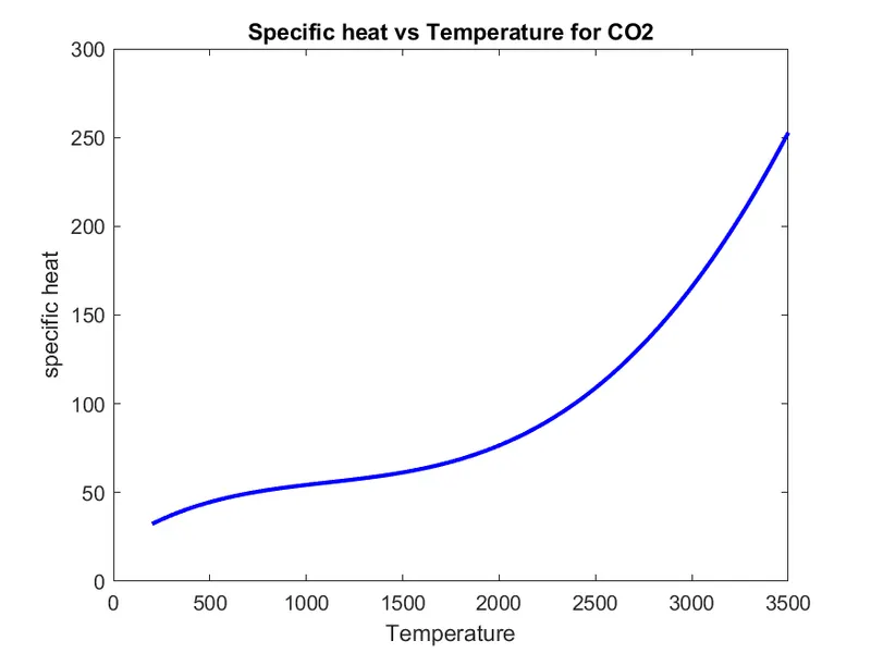
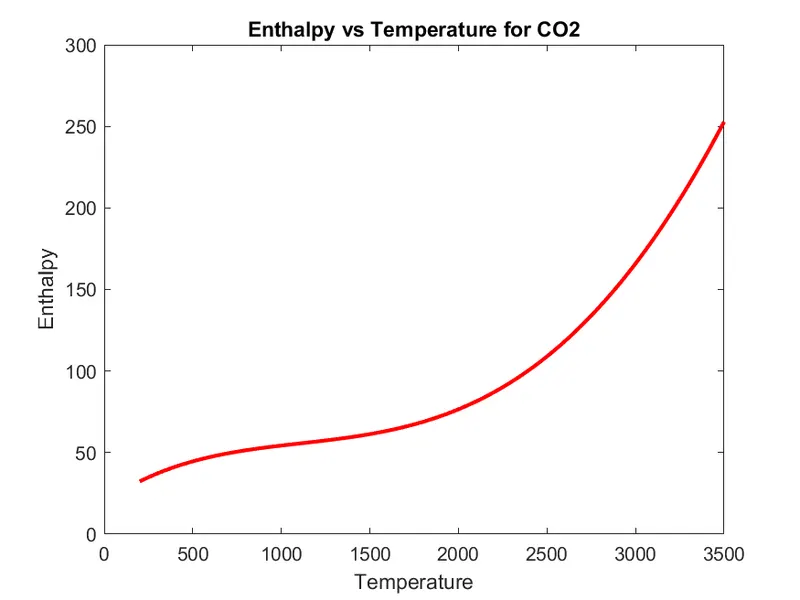
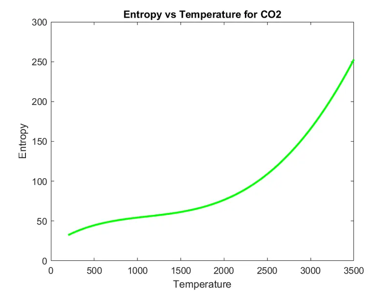
3. To plot the cp, Enthalpy and Entropy for the local temperature range specific for each species save the plots as image with the appropriate names and dump them in separate folders for each species with suitable name.

THEORY:

• Thermodynamics data for individual species are necessary for performing equilibrium chemistry and finite-rated chemical kinematics calculations.
• These data typically provide the thermodynamics properties (enthalpy,entropy,specific heat) of a species as a function of temperature.
• Thermodynamics data for individual species are requried in many applications involving chemical reactions. For over 50 years NASA lewis(now Glenn) research center has been compiling and disseminating thermodynamics data for use in its chemical equilibrium programs.
• These data, wisely used for thermodynamics community have grown from 42 species to current 2000. For calculation purpose, the use of thermodynamics data in the form of simple empirical equations has some obvious advantages.
• First,it makes tabular interpolation and third it condense all the tabular information into a few constants that accurately reproduce the many thermodynamics data points.

ENTHALPY(h):

Enthalpy(h) is the sum of the internal energy of the system plus the product of the pressure of the gas in the system and its volume: H=U+PV. Therefore, enthalpy of a gas decreases with pressure at constant temperature. Enthalpy of the liquid phase at constant temperature remains the same for moderate pressures. For a process at the constant pressure the change of enthalpy is

`h/(RT)=a1+a2.T/2+a3.T^2/3+a4.T^3/4+a5.T^4/5+(a6)/T`

where,

h=enthalpy,

R=universal gas constant,

T=temperature,

a=co-efficients.

ENTROPY(S):

`s/(R)=alnT+a2.T+a3.T^2/2+a4.T^3/3+a5.T^4/4+a7`

where,

s=entropy.

Where `del`qrev is the reverisable heat flow. When a fluid system changes from state A to state B by an irreversiable process, then the change of its entropy is be `triangle`S = SB-SA.

SPECIFIC HEAT(cp):

The specific heat (cp) is the amount of heat per unit mass required to raise the temperature by one degree celcius.The specific heat of water is 1 calorie/gram degree celsius which is higher than any other common substance.

`cp/(R)=a1+a2.T+a3.T^2+a4.T^3+a5.T^4`

GOVERNING EQUATIONS USED:

Here,

• R is a universal gas constant ,
• T is the temperature,

The 1st 7 co-efficients are HIGH TEMPERATURE co-efficients and 2nd 7 co-efficients are LOW TEMPERATURE co-efficients.

BODY OF THE CONTENT:

• main code
• code for: 1.specific heat 2.enthalpy 3.entropy and 4.molecular weight
• plotting.

MATLAB CODE:

code for main program:

%A program code for parsing the given data and calculate various thermodynamics

close all 
clear all
clc

f1=fopen('THERMO.dat','r');
first_line=fgetl(f1);

%global temperature
global_temp =fgetl(f1);
temp_range = strsplit(global_temp," ");
global_low_temp  = str2double(temp_range{2});
global_mid_temp  = str2double(temp_range{3});
global_high_temp = str2double(temp_range{4});


%skipping the lines
for i=1:3
    remove = fgetl(f1);
end

for i=1:53
    %calculating local temp species
    local_temp_range= fgetl(f1);
    D= strsplit(local_temp_range,' ')
    local_low_temp= str2double(D{end-3});
    local_mid_temp=str2double(D{end-1});
    local_high_temp=str2double(D{end-2});
    
    name=D{1};
    T= linspace(local_low_temp,local_high_temp,400);
    R= 8.314;

    line1= fgetl(f1);
    line2= fgetl(f1);
    line3= fgetl(f1);
    
    
    A=strfind(line1,'E');
    B=strfind(line2,'E');
    C=strfind(line3,'E');

    a1= str2num(line1(1:A(1)+3));
    a2= str2num(line1(A(1)+4:A(2)+3));
    a3= str2num(line1(A(2)+4:A(3)+3));
    a4= str2num(line1(A(3)+4:A(4)+3));
    a5= str2num(line1(A(4)+4:A(5)+3));
    a6= str2num(line2(1:B(1)+3));
    a7= str2num(line2(B(1)+4:B(2)+3));


   
    b1= str2num(line2(B(2)+4:B(3)+3));
    b2= str2num(line2(B(3)+4:A(4)+3));
    b3= str2num(line2(B(4)+4:A(5)+3));
    b4= str2num(line3(1:C(1)+3));
    b5= str2num(line3(C(1)+4:C(2)+3));
    b6= str2num(line3(C(2)+4:C(3)+3));
    b7= str2num(line3(C(3)+4:C(4)+3));

    cp= specificheat(a1,a2,a3,a4,a5,b1,b2,b3,b4,b5,T,R,local_mid_temp);

    h= enthalpy(a1,a2,a3,a4,a5,a6,b1,b2,b3,b4,b5,b6,T,R,local_mid_temp);

    s= entropy(a1,a2,a3,a4,a5,a7,b1,b2,b3,b4,b5,b7,T,R,local_mid_temp);

    Molecular_wt(i)= molecular_weight(name);

    plotting(cp,h,s,T,name)

end

code explanation for main program :

• To read the given, fopen command was used and fget command was used to read the subsequent lines,which is headers to comments and numerical entries.
• To extract the numerical values of global and local temperatures which were stored as string by using split the given line according to spaces provided in between of them and were converted from string to double datatype using str2double command and were stored in respective variables.
• The total number of variables no.of.species present in the given data file was 53, so for loop was initiated from 1 to 53 times for reading each species and 14 co-efficients were present under each species.These co-efficients are again extracted and converted from string to double datatype.
• Two seperate functions for molecular weight and specific heat,enthalpy,entropy were created which is stored the required data and formulas for calculation.
• The functions created were called in main program for further calculations and respective graphs were plotted to specific heat, enthalpy, entropy, w.r.t time for each species were obtained.

code for plotting:

function plotting(cp,h,s,T,name)
cd(pwd)
dir_name=name;
mkdir(dir_name);

figure(1)
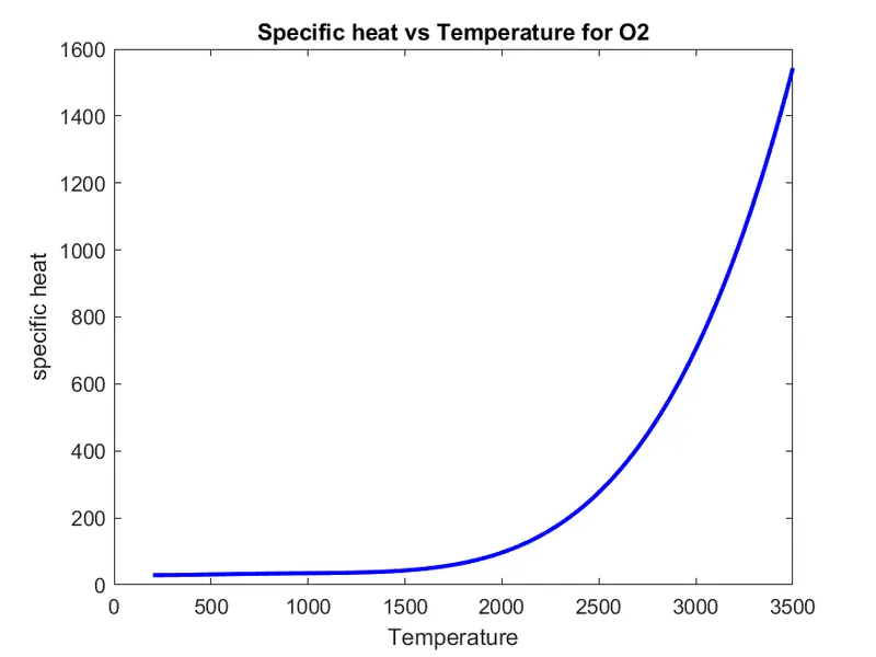
plot(T,cp,'LineWidth',2,'Color','b')
title(sprintf('Specific heat vs Temperature for %s',name))
xlabel('Temperature')
ylabel('specific heat')

figure(2)
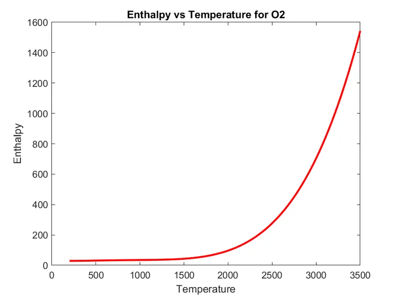
plot(T,cp,'LineWidth',2,'Color','r')
title(sprintf('Enthalpy vs Temperature for %s',name))
xlabel('Temperature')
ylabel('Enthalpy')

figure(3)
plot(T,cp,'LineWidth',2,'Color','g')
title(sprintf('Entropy vs Temperature for %s',name))
xlabel('Temperature')
ylabel('Entropy')

cd(dir_name)
   saveas(1,'cp_vs_t.png')
   saveas(2,'h_vs_t.png')
   saveas(3,'s_vs_t.png')
   cd ..
end

EXPLANATION:

• Then, we plot the code for the main to get the graph.The command mkdir() is used to save the program file in the seperate folders.
• The folders for the each species that have contains the graphs for specific heat, temperature, entropy, enthalpy.
• As well as, we should give the perfect title to identify the each folder to define each one of the species.

code for entropy(s):

function s= entropy(a1,a2,a3,a4,a5,a7,b1,b2,b3,b4,b5,b7,T,R,local_mid_temp);

if T<=local_mid_temp
    s=R*(a1.*log(T)+a2.*T+a3.*(T.^2)./2+a4.*(T.^2)./3+a5.*(T.^2)./4+a7);
else
    s=R*(b1.*log(T)+b2.*T+b3.*(T.^2)./2+b4.*(T.^2)./3+b5.*(T.^2)./4+b7);
end

EXPLANATION:

• The code for entropy that contains the formula as we mentioned below, the program and also we applied the conditions Temperature should be less than or equal to local_mid_temperature.

code for enthalpy(h):

function h= enthalpy(a1,a2,a3,a4,a5,a6,b1,b2,b3,b4,b5,b6,T,R,local_mid_temp);

if T>local_mid_temp
    h= R.*T.*(a1.*T+(a2.*T.^2)./2+(a3.*T.^3)./3+(a4.*T.^4)./4+(a5.*T.^5)./5+a6);

else
     h= R.*T.*(b1.*T+(b2.*T.^2)./2+(b3.*T.^3)./3+(b4.*T.^4)./4+(b5.*T.^5)./5+b6);

end

EXPLANATION:

• As also enthalpy we have a formula to be used and with the different condition. The temperature must greater than the local_mid_temperature.

code for specific heat(cp):

function cp= specificheat(a1,a2,a3,a4,a5,b1,b2,b3,b4,b5,T,R,local_mid_temp)

if T>local_mid_temp
    cp=R.*(a1+a2.*T+a3.*T.^2+a4.*T.^3+a5.*T.^4);

else
    cp=R.*(b1+b2.*T+b3.*T.^2+b4.*T.^3+b5.*T.^4);
end

EXPLANATION:

• The specific heat is also similar to the condition that we used for the enthalpy but, the formula was different as per the formula mentioned below.

code for molecular weight:

function MW = molecular_weight(name)
atoms=['H','C','O','N','R'];
fprintf('molecular weight of');
fprintf(name);
fprintf(':');
atomic_weight=[1 12 16 14 40];
MW=0;
for i=1:length(name)
    for j=1:length(atoms)
        if strcmp(name(i),atoms(j))
            MW=MW+atomic_weight(j);
            position=j;
        end
    end
    n=str2double(name(i));
    if n>1
        MW=MW+atomic_weight(position)*(n-1);
    end
end
fprintf('%d \n',MW);
disp('');
end

EXPLANATION:

• This important code to plot all the main code and it will display the maolecular weight for the given species in NASA thermodynamics.
• And also,we search for atomic weight for the taken species in the internet to find the molecular weight for the species for over 200 species .

RESULTS:

File parsing of nasa thermodynamics data was done sucessfully.

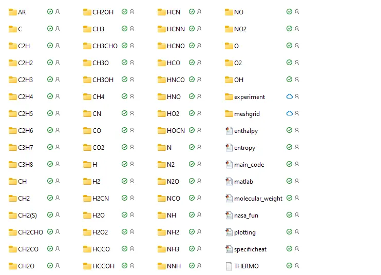
MOLECULAR WEIGHT OUTPUTS:

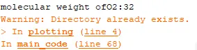
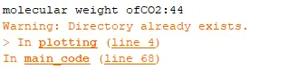
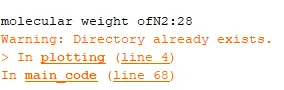
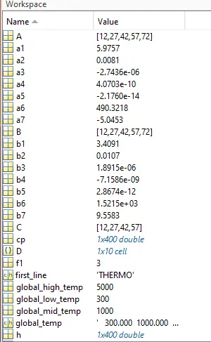
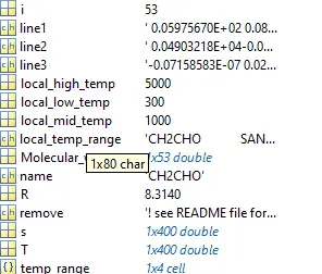
WORKSPACE OUTPUTS:

PLOTS FOR O2,N2,CO2 SPECIES:

GOOGLE DRIVE LINK:

https://drive.google.com/drive/folders/196YO5OcZgIQTYISCFKjKun6pqKQz_dFF

CONCLUSION:

Using matlab code, the neccessary co-efficients required to evaluate various thermodynamics parameters for different species are extracted from NASA thermodynamics data file is calculated and plotted the graph.The specific heat, enthalpy, and entropy for all the species are calculated and plotted against the local temperature range. The molecular weight is calculated for all the species.