Challenge

Week 4.1 - Genetic Algorithm

MMd Zafar Hayat25 May 2022

Our objective is

1) Write a code in MATLAB to optimise the stalagmite function and find the global maxima of the function.

2) Plot graphs for all 3 studies and for F maximum vs no. of iterations.

Approach stragedy

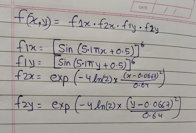
The function is already given in video of stalagmite, so here we directly explain the coding and function of required and for that I will do 4 coding 1st is for global maxima 2nd is for function i.e stalagmite 3rd is for studies 4th is also a function but for minima.

WRITING CODE OF GLOBAL MAXIMA

FIRST OF ALL I STARTED WITH

clear all {clear the workspace if it has data of earlier coding}

close all {close all the plots if opened in background}

clc {clear the command windows}

THEN I WROTE

x=linspace(0,0.6,151); {creating x values in 151 equal interval of range 0 to 0.6 by using linspace cmd}

y=linspace(0,0.6,151); {creating y values in 151 equal interval of range 0 to 0.6 by using linspace cmd}

[xx,yy]=meshgrid(x,y); {create 2D array by using meshgrid command for each x and y and stored in xx and yy}

THEN I WROTE

for i=1:length(xx) {starting for loop by using i from 1 to length of xx}

for j=1:length(yy) {starting for loop by using i from 1 to length of yy}

input_vector(1)=xx(i,j);

input_vector(2)=yy(i,j);

{here xx(i,j) & yy(i,j) are element of matrix in x and y for values of i and j & stored in input_vector "(1) represents 1st matrix and (2) represent 2nd matrix of input_vector}

f(i,j)=stalagmite(input_vector); {it basically uses stalagmite function and stored "f" for each value for i and j & I have created stalagmite function which I will discuss further}

end

{end of the loop}

THEN I WROTE

surfc(xx,yy,f) {this cmd is used to plot the counter surface by using xx,yy,f datas}

xlabel('X-Axis')

ylabel('Y-Axis')

{lebelling the x and y coordinate respectively}

shading interp {this is used to make smooth curve coloring rather than grid lines on it}

THEN I WROTE

[inputs,fval]=ga(@stalagmite,2); {this cmd is basically stores x value in inputs & y values in fval and ga is inbuilt function which gives minima of function}.

SOME DISCUSSION ABOUT GA FUNCTION

The format of ga command is

[abc,xyz]=ga(function,nvars,A,B,A',B',lb,ub,nonicon,Intcon,options)

here,

abc is x value and xyz is y values

in bracket there is function which takes function name which was built in saperately

nvars is the no. of variables

A & B are is used in case linear inequality constrain is of the type A*x<B, if nothing enter[]

A' & B' are is used in case linear inequality constrain is of the type A*x=B, if nothing enter[]

lb & ub they provide the search space for GA it is basically lower limit and upper limit in GA, if left blank it will search beyond search space

nonicon set non linear constrain if any

Intcon set integer constrain if any

options to change any default GA functioning, eg using 50 it will run upto 50 values

WRITING CODE OF STALAGMITE FUNCTION

the function to be code is below

function question_given=stalagmite(input_vector) {making stalagmite function and input is input_vector & assigning it to question_given}

x=input_vector(1);

y=input_vector(2);

{input_vector(1) represents matrix's 1st element and input_vector(2) represents matix's 2nd element and assigned to x and y respectively}

fn1x=(sin((5.1*pi*x)+0.5))^6;

fn1y=(sin((5.1*pi*y)+0.5))^6;

fn2x=exp((-4*log(2)/0.64)*((x-0.0667)^2));

fn2y=exp((-4*log(2)/0.64)*((y-0.0667)^2));

{splitting each term into saperate name as shown above}

question_given=fn1x*fn1y*fn2x*fn2y; {multiplying each term and stored it in question_given}

end {ending the function}

THE CODE IS ATTACHED BELOW

clear all
close all
clc


x=linspace(0,0.6,151);
y=linspace(0,0.6,151);

[xx,yy]=meshgrid(x,y);

for i=1:length(xx)
    for j=1:length(yy)
        input_vector(1)=xx(i,j);
        input_vector(2)=yy(i,j);
        f(i,j)=stalagmite(input_vector);
    end
end


surfc(xx,yy,f)
xlabel('X-Axis')
ylabel('Y-Axis')

shading interp

[inputs,fval]=ga(@stalagmite,2);

STALAGMITE FUNCTION CODE

function question_given=stalagmite(input_vector)

x=input_vector(1);
y=input_vector(2);

fn1x=(sin((5.1*pi*x)+0.5))^6;
fn1y=(sin((5.1*pi*y)+0.5))^6;
fn2x=exp((-4*log(2)/0.64)*((x-0.0667)^2));
fn2y=exp((-4*log(2)/0.64)*((y-0.0667)^2));
question_given=fn1x*fn1y*fn2x*fn2y;
end

"I have run above code 3 times and the results came same as earlier plz find all 3 plots attached"

Plot graphs for all 3 studies and for F maximum vs no. of iterations

For global maxima we use "question_given=fn1x*fn1y*fn2x*fn2y;"

For global minima we use "question_given=-fn1x*fn1y*fn2x*fn2y;"

WRITING CODE OF GLOBAL MINIMA

\\ plz note this code I have got helped from sarang sir video named stalagmite HW \\

clear all
close all
clc

x=linspace(0,0.6,151);
y=linspace(0,0.6,151);

[x,y]=meshgrid(x,y);
num_case=50;
f=global_minima(x,y);

tic

%study1 statistical behaviour
for i=1:num_case
    [inputs,fopt(i)]=ga(@stalagmite,2);
    xopt(i)=inputs(1);
    yopt(i)=inputs(2);
end

running_time=toc

%ploting 1
figure(1)
subplot(2,1,1)
hold on
surfc(x,y,f)
shading interp
plot3(xopt,yopt,fopt,'marker','o','markersize',5)
title('Unbounded inputs')
subplot(2,1,2)
plot(fopt)
xlabel('Iteration')
ylabel('function Minimum')

tic

%study2- Statistical behaviour

for i=1:num_case
    [inputs,fopt(i)]=ga(@stalagmite,2,[],[],[],[],[0,0],[0.4,0.4],[],[]);
    xopt(i)=inputs(1);
    yopt(i)=inputs(2);
end

running_time=toc

%ploting 2
figure(2)
subplot(2,1,1)
hold on
surfc(x,y,f)
shading interp
plot3(xopt,yopt,fopt,'marker','o','markersize',5)
title('bounded inputs')
subplot(2,1,2)
plot(fopt)
xlabel('Iteration')
ylabel('function Minimum')

%increasing ga iteration
options=optimoptions('ga')
options=optimoptions(options,'populationsize',170)

tic

for i=1:num_case
    [inputs,fopt(i)]=ga(@stalagmite,2,[],[],[],[],[0,0],[0.4,0.4],[],[],options);
    xopt(i)=inputs(1);
    yopt(i)=inputs(2);
end

running_time=toc

%ploting 3
figure(3)
subplot(2,1,1)
hold on
surfc(x,y,f)
shading interp
plot3(xopt,yopt,fopt,'marker','o','markersize',5)
title('bounded inputs')
subplot(2,1,2)
plot(fopt)
xlabel('Iteration')
ylabel('function Minimum')

function question_given=global_minima(x,y)
fn1x=(sin((5.1*pi*x)+0.5)).^6;
fn1y=(sin((5.1*pi*y)+0.5)).^6;
fn2x=exp((-4*log(2)/0.64).*((x-0.0667).^2));
fn2y=exp((-4*log(2)/0.64)*((y-0.0667).^2));
question_given=-fn1x.*fn1y.*fn2x.*fn2y;
end

All above 3 cases have same coding the difference is only the minute changes, so I will explain only one case and if there is any minute changes came i will explain that also.

I have started with clear all, close all, clc this cmd is already discussed in 1st coding then I created x and y matrix by using linspace cmd of 151

then i created matrix of 151x151 by using meshgrid cmd and stored in [x,y], then i assigned 50 to num_case and wrote f=global_minima(x,y),after that i used tic this is for starting of time after that I used for loop with i=1:num_case then I wrote [inputs, fopt(i)]=ga(@stalagmite,2) here input is x and fopt(i) always changes the each loop , 2 is no. of variable after that I wrote xopt(i) & yopt(i) this always changes with each loop and stored in input(1) and input(2) respectively in matrix form after that I ended for loop and ended time by using toc cmd and stored in running_time.

Then I started with figure(1) which is used to naming plot windows further I wrote subplot(2,1,1) here 2 stands for no. of grid row,1 stands for no. of grid column & 1 stands for grid position of new axes.

hold on cmd is used to hold plot by keeping old lines and also keeping new lines then surf cmd is used to plot surface of counter figure then I used shading inturpt which make smooth color and disappear the grid lines afterward plot3 cmd is used to create 3d space lines by using xopt,yopt, fopt as variable then I put title then again subplot afterward plot(fopt) is used to plot fopt variable finally lebelling the x and y axis given above.

this whole things is used in all 3 studies there is but minute difference is in 3rd case that is

options=optimoptions('ga')

options=optimoptions(options,'populationsize',170)

this cmd is used to make population size of 170 and stored in options rest are all same

\\plz find attached plot of all 3 studies

Week 4.1 - Genetic Algorithm

Ship work like this
in your own course.

Talk to a career counsellor

Ship work like thisin your own course.

Talk to a career counsellor

Ship work like this
in your own course.