Project 2 - Rankine cycle Simulator

Our Aim is to:- Create a Rankine Cycle Simulator using OCTAVE/MATLAB (of any choice).

Given datas:-

Turbine Inlet temperature = 400° C

Turbine Inlet Pressure = 30 bars

Turbine Outlet Pressure = 0.05 bars = Condenser Inlet Pressure

Some briefly comment about Rankine cycle

Basically this cycle is work producing type cycle where we can extract work from it.

It basically consist of 4 devices with each device have some working properties,

1st device:- BOILER-> heat is added to water at constant pressure by burning of coal or by radioactive uranium fission.

2nd device:- TURBINE-> the superheated steam (whose temp. is very greater than boiling point, say 400 deg cel) at high temp & pressure expands at isentropic expansion and at exit, temp. & pressure drops very high amount. It consist of moving blade which got rotate by expansion through which we get rotational kinetic energy.

3rd device:- CONDENSER->heat is rejected at constant pressure by passing water through shell which is at ambient.

4th device:- PUMP-> this help the water which is saturated liquid to increase the pressure by pumping to boiler from condenser & the process executes is isentropic compression.

The above 4 devices have thermodynamical path shown in red color that only constitutes the rankine cycle in diagrams.

Rankine cycle T-S Diagram

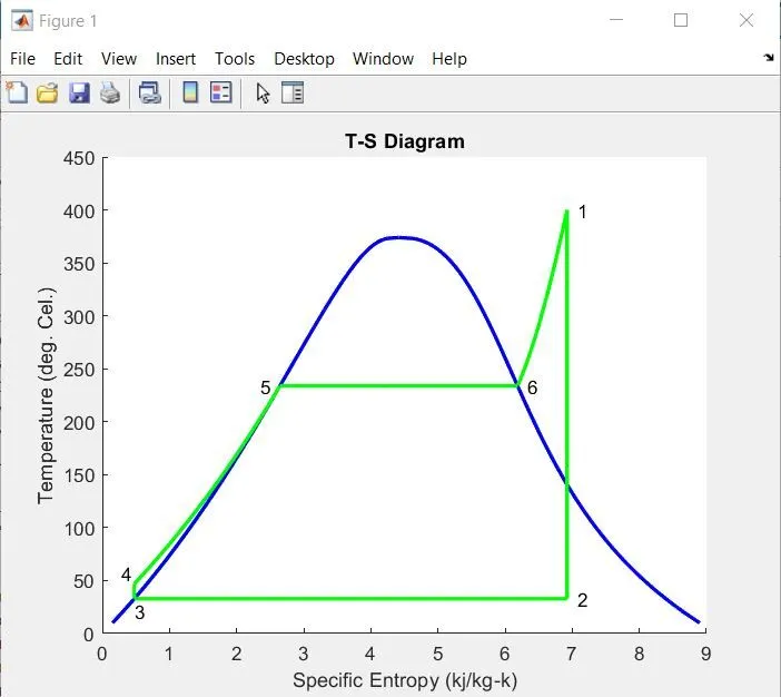
Here,

1-2 is TURBINE , 2-3 is CONDENSER, 3-4 is PUMP, 4-5-6-1 is BOILER.

the blue line shown here is saturated line, in which area within line is wet region, outer side of saturated line left hand side is liquid region, outer side of saturated line right hand side is vapour region.

3-2 have constant pressure of 0.05 bars & in T-S diagram const pressure line is curve in nature but here in T-S diagram it is shown straight, because the line is in wet region & in this region "Latent Heat of Vaporization" came into picture, whose work is to change phase of substance (from liq<=>gas and vice versa) so temp remains const entropy increases/decrease.

Similarly,

this explanation holds good for 5-6 the change is only here pressure is 30 bars, so this line is above 3-2.

For 4-5 pressure is still 30 bars but this line is in liquid region for that "constant pressure heat of liquid" came into picture, whose work is to increase temperature at const pressure of substance.

For 6-1 pressure is still 30 bars but this line is in vapour region for that "constant pressure heat of vapour" came into picture, whose work is to increase temperature at const pressure of substance.

CODING TIME:-

So I started with

then I wrote

s1=XSteam('s_pT',p1,t1); {here XSteam('s_pT',p1,t1) gives sp. entropy at pressure p1 & temp t1 & stored in s1}

h1=XSteam('h_pT',p1,t1); {here XSteam('h_pT',p1,t1) gives sp. enthalpy at pressure p1 & temp t1 & stored in h1}

t2=XSteam('Tsat_p',p2); % Saturation Temperature at 0.05 bar {here this cmd gives saturation temp at pressure p2}

t3=t2; {assigning t2 value to t3}

s2=XSteam('sV_p',p2);

h2=XSteam('hV_p',p2);

s3=XSteam('sL_p',p2);

h3=XSteam('hL_p',p2);

v3=XSteam('vL_p',0.05);

{similarly in this way I have extracted value of s2,h2,s3,h3,v3 & all have same explanation as explained before}

then I wrote

\\above shown is basic thermodynamic formula of work absorbing device say pump, here v denotes specific volume at entrance to pump inlet, P2 is higher pressure, P1 is lower pressure (p should be in kilopascals)\\

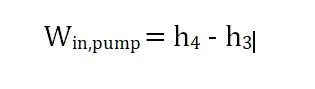
work_pump=v3.*((p1-p3).*100); % gives in kj/kg {here basically I have written formula for pump & multipiled by 100 for converting bar to kpa}

h4=work_pump+h3; {finding enthalpy at point 4 by using above formula}

h5=XSteam('hL_p',p1); {here we have find enthalpy at point 5}

h6=XSteam('hV_p',p1); {here we have find enthalpy at point 6}

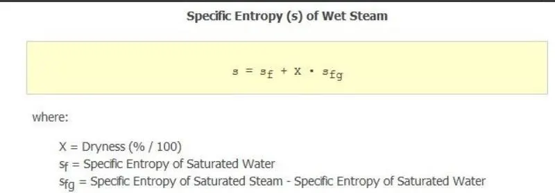
x=((s1-s3)/(s2-s3)); {at pressure 0.05 s=s1, s2 is s-vapour, s1 is s-liquid, by using this I have used above formula to find x}

wet_h2=XSteam('h_px',p2,x); {finding wet region enthalpy at poinnt 2}

s5=XSteam('sL_p',p1); {finding enthalpy at point 5}

s6=XSteam('sV_p',p1); {finding enthalpy at point 6}

s4=s3; {assigning s3 value to s4}

cpL_p1=XSteam('CpL_p',p1); {here I have found constant heat pressure in liquid region at pressure p1}

t5=XSteam('Tsat_p',p1); % Saturation Temperature at 30 bar {finding saturation temp at pressure p1}

t6=t5; {assigning t5 value to t6}

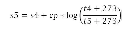
t4=(((t5+273)/(exp((s5-s4)/cpL_p1)))-273); {finding t4 on basis of above given formula}

then I wrote

crict_temp=XSteam('Tsat_p',220.63949); {finding critical temp at pressure 220.63949 & storing crict_temp}

tempup=linspace(10,crict_temp,401); {creating 401 equal interval between 10 & crict_temp and storing in tempup}

tempdown=linspace(crict_temp,10,401); {creating 401 equal interval between crict_temp & 10 and storing in tempdown}

then I wrote

for i=1:401 {starting for loop with i from 1 to 401}

sp_entropy_up(i)=XSteam('sL_T',tempup(i)); {collecting saturated liquid line datas in matrix}

sp_entropy_down(i)=XSteam('sV_T',tempdown(i)); {collecting saturated vapour line datas in matrix}

end {end of loop}

then I wrote

figure(1) {assigning 1st plot}

hold on {cmd enables to hold the line on plot}

plot(sp_entropy_up,tempup,'Color','b','LineWidth',2) {plotting saturated liquid curve}

plot(sp_entropy_down,tempdown,'Color','b','LineWidth',2) {plotting saturated vapour curve}

xlabel('Specific Entropy (kj/kg-k)') {lebelling the x axis}

ylabel('Temperature (deg. Cel.)') {lebelling the y axis}

axis([0 9 0 450]) {fixing the axis coordinate}

title('T-S Diagram') {giving title to the diagram}

then I wrote

% Process 1-2

t_variable1=linspace(t1,t2,501); {creating 501 equal interval between t1 & t2 and storing in t_variable1}

s_variable1=linspace(s1,s1,501); {creating 501 equal interval between s1 & s1 and storing in s_variable1}

plot(s_variable1,t_variable1,'Color','g','LineWidth',2) {creating plot by using above 2 variable}

text(s1+0.15,t1,'1') {adding text to different spot of plot in this case it is 1}

then I wrote

% Process 2-3

s_low_pr=linspace(s3,s1,201);

t_low_pr=linspace(t3,t3,201);

plot(s_low_pr,t_low_pr,'Color','g','LineWidth',2)

text(s1+0.15,t2,'2')

% Process 3-4

t_variable2=linspace(t3,t4,301);

s_variable2=linspace(s3,s4,301);

plot(s_variable2,t_variable2,'Color','g','LineWidth',2)

text(s3,t2-12,'3')

{same explanation as explained above 1-2 process}

then I wrote

% Process 4-5

t4_varies=linspace(t4,t5,501); {creating 501 equal interval between t4 & t5 and storing in t4_varies}

s4_to_s5=s5-cpL_p1.*(log((t5+273)./(t4_varies+273))); {it is basically assigning values in formula pasted few line above}

plot(s4_to_s5,t4_varies,'Color','g','LineWidth',2) {creating plot by using above 2 variable}

text(s4-0.2,t4+10,'4') {adding text to different spot of plot in this case it is 4}

then I wrote

% Process 5-6

s_high_pr=linspace(s5,s6,201);

t_high_pr=linspace(t5,t6,201);

plot(s_high_pr,t_high_pr,'Color','g','LineWidth',2)

text(s5-0.3,t5,'5')

{the explanation of above 4 lines is exactly similar to above explained 1-2 process}

then I wrote

% Process 6-1

p_varies=linspace(p1,p1,301);

t_varies=linspace(t6,t1,301); {these 2 lines creates equal 301 interval of pressure and temp and stores in p_varies & t_varies respectively}

for i=1:301 {starting the for loop with i =1 to 301}

s6_to_s1(i)=XSteam('s_pT',p_varies(i),t_varies(i)); {storing the data for each loop turn}

end {ending of loop}

plot(s6_to_s1,t_varies,'Color','g','LineWidth',2) {plotting the entropy and temp from 6 to 1}

text(s6+0.15,t6,'6') {adding text to different spot of plot in this case it is 6}

then I wrote

figure(2) {setting up new plot}

hold on {holding up the plot lines}

for i=1:401 {starting for loop with i=1 to 401}

sp_enthalpy_up(i)=XSteam('hL_T',tempup(i)); {creating data for h-s diagram saturated liquid line}

sp_enthalpy_down(i)=XSteam('hV_T',tempdown(i)); {creating data for h-s diagram saturated vapour line}

end {ending of loop}

plot(sp_entropy_up,enthalpy_up,'Color','b','LineWidth',2) {plotting saturated liquid line}

plot(sp_entropy_down,enthalpy_down,'Color','b','LineWidth',2) {plotting saturated vapour line}

xlabel('Specific Entropy (kj/kg-k)') {lebelling x axis}

ylabel('Specific Enthalpy (kj/kg)') {lebelling y axis}

axis([0 10 -50 4500]) {constraining the axes}

title('Enthalpy-Entropy Diagram') {giving the title}

then I wrote

%process 1-2

p_varies=linspace(p1,p2,501);

for i=1:501

p_variable(i)=p_varies(i);

s_varies(i)=s_variable1(i);

h1_to_h2(i)=XSteam('h_ps',p_variable(i),s_varies(i));

end

plot(s_varies,h1_to_h2,'Color','g','LineWidth',2)

text(s1+0.15,h1,'1')

% Process 2-3

p_varies=linspace(p2,p3,501);

s_variable1=linspace(s1,s3,501);

for i=1:501

p_variable(i)=p_varies(i);

s_varies(i)=s_variable1(i);

h2_to_h3(i)=XSteam('h_ps',p_variable(i),s_varies(i));

end

plot(s_varies,h2_to_h3,'Color','g','LineWidth',2)

text(s1+0.15,wet_h2,'2')

%process 3-4

p_varies=linspace(p2,p1,301);

for i=1:301

p_variable1(i)=p_varies(i);

s_varies2(i)=s_variable2(i);

h3_to_h4(i)=XSteam('h_ps',p_variable1(i),s_varies2(i));

end

plot(s_varies2,h3_to_h4,'Color','g','LineWidth',2)

text(s3,h3-65,'3')

%process 4-1

p_varies=linspace(p1,p1,501);

s_variable1=linspace(s4,s1,501);

for i=1:501

p_variable(i)=p_varies(i);

s_varies(i)=s_variable1(i);

h4_to_h1(i)=XSteam('h_ps',p_variable(i),s_varies(i));

end

plot(s_varies,h4_to_h1,'Color','g','LineWidth',2)

text(s4,h4+120,'4')

\\ Above all process i.e 1-2, 2-3, 3-4, 4-1 have same plan of approach that is I have used linspace for creating equal interval matrix for both pressure & entropy saperately then I started for loop ran from 1 to 501 times as well as 1 to 301 times according to condition I chosen, within it I assign each value of created linspace values to new variable for both pressure and entropy & also I have used that new outcame values to XSteam & assign new variable to XSteam for each loop turn,

finally I plotted new value of XSteam & entopy generated, afterward I wrote each process a new text, i.e 1,2.... in this way I can achieve my graphs for h-s \\

% Calculation of reqired datas

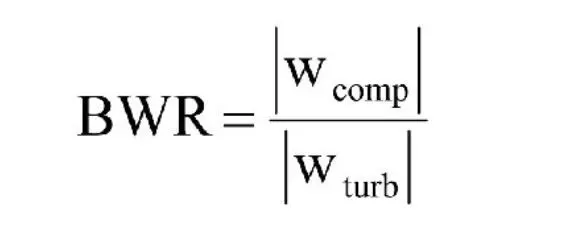
back_work_ratio=((h4-h3)/(h1-wet_h2)); {I have used formula & shown above and wrote formula accordingly}

a=sprintf('Back Work Ratio is %f',back_work_ratio); {this whole cmd converts into string and saved into 'a'}

net_work_output=((h1-wet_h2)-(h4-h3)); {I have used formula & shown above and wrote formula accordingly}

b=sprintf('Net Work Output (Wturbine- Wpump) is %f',net_work_output); {this whole cmd converts into string and saved into 'b'}

helpdlg(b); {this cmd enable to give output a dialog box with values displayed inside box here it will give 'b value'}

msgbox(a); {this cmd enable to give output a dialog box with values displayed inside box here it will give 'a' value}

efficiency= ((h1-h2)-(h4-h3))/(h1-h4) {writting efficiency formula from thermo text books}

\\plz note I have used 2 different cmd i.e helpdlg & msgbox I did this because at one time either of one can't show 2 value simultaneously\\

WHAT I HAVE RESEARCHED:-

• As I observed that turbine exit is in wet region it means that water vapour and water liquid together will hit the blade of turbine this means the corosion of blade is likely to be very high & its life would be fall down very rapidly.
• The efficiency of rankine cycle will always 35% to 45% it can't be 100% because it will break the law of thermodynamics i.e conversion of heat to work 100% is impossible.
• I just checked by altering pressure temp which is given in question then I got multiple plot & efficiency in which came up with optimum temp to get max work i.e at 900 deg celsius (plz find reasearch 1.jpg) in which it max max efficiency without causing too much loss of heat, means available energy is more according to basic of thermodynamics & research 2.jpg is original data given with efficiency in challenge plz compare it.
• Few research detail I have noted in paper (I am attaching it flz find by name) there we can see mutliple process so we increase performance of rankine cycle.

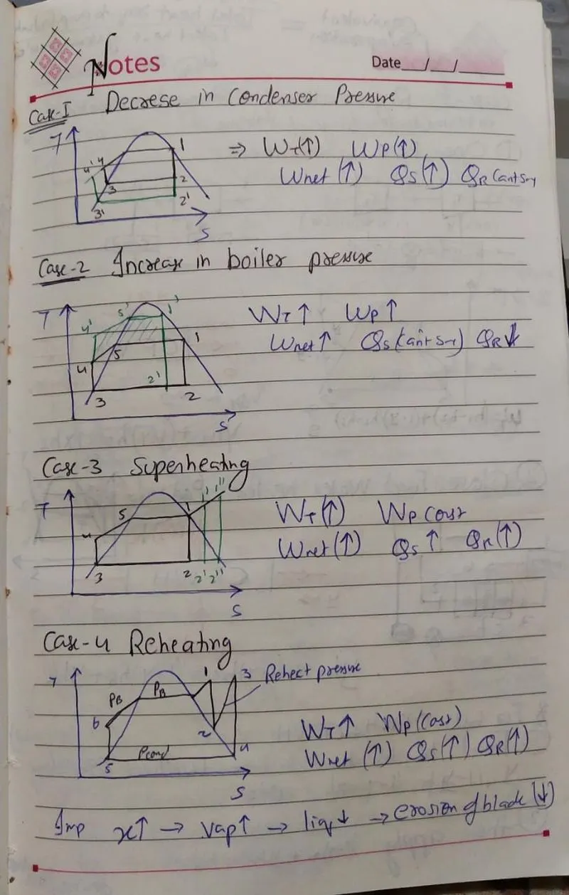
\\ here

Wt- refers to work produced by turbine

Wp- refers to work absorbed by pump

Wnet is Wt-Wp

Qs- refers to heat supply to boiler

Qr- refers to heat rejected in atmosphere by condenser

Up arrow- refers increasing

down arrow- refers decreasing

x is dryness fraction \\