Week 3 - Solving second order ODEs
Our objective is to "Write a program that solves the above ODE, & Create movie of motion of Pendulum.
So,
basically I created seperate function under named "challenge_ode" and then used it in our main programme.
WRITTING OUR MAIN PROGRAMME
I started with
clear all {this command enables clear the workspace if earlier have some data}
close all {this command enables close the plots if some plots are open in background}
clc {this command enables clear the command window if earlier have some data}
after that i wrote
b=0.05; {b is assigned a value of 0.05 which is damping co-efficient in our equation}
g=9.81; {g is assigned a value of 9.81 which is gravity}
l=1; {l is length of pendulum rod which have given value of 1 meter}
m=1; {m is mass of bob which is 1 kg}
after that i wrote
theta_initial=[0;3]; {It is initial condition given in problem "0" is angular displacement and "3" is angular velocity, and I have assigned in matrix form to "theta_initial"}
after that i wrote
time_duration=linspace(0,20,501) {In our problem it is given that integretion time is from 0 to 20 seconds thatswhy I have used linspace(0,20,501) this cmd generates 501 values range from 0 to 20 in equal interval}
after that i wrote
[t, results]=ode45(@(t,theta) challenge_func(t,theta,b,g,l,m),time_duration,theta_initial);
{here ode45 is command used to solve differential eqn in matlab & (@(t,theta) basically tells that our main inputs are t and theta, challenge_func(t,theta,b,g,l,m) came from function which I wrote seperately,time_duration is range of integration, theta_initial is initial condition}
after that i wrote
figure(1) {this is used to make seperate plot window}
plot(t,results(:,1),"Color",'b','LineWidth',1.5) {as we know results is 501 X 2 matrix thats why I wrote x coordinate="t" & y coordinate=results(:,1)[: represent whole row & 1 represent 1st column]}
hold on {this cmd used in printing both figures because if it is not written then it will print latest command}
plot(t,results(:,2),"Color",'r','LineWidth',1.5){as we know results is 501 X 2 matrix thats why I wrote x coordinate="t" & y coordinate=results(:,2)[":" represent whole row & "2" represent 2nd column]}
xlabel('Time in Seconds') {lebelling the x axis}
ylabel("Angular Displacement & Angular Velocity") {lebelling the x axis}
legend('Angular Displacement','Angular Velocity') {this cmd is used to make lebelling which lines stands for what}
NOTE:- As we know the results are angular displacement & angular velocity therefore we should write sin instead of sind because it is in radian.
after that i wrote
x=l*sin(results(:,1)); {gives x-coordinate in cartesian of pendulum}
y=l*cos(results(:,1)); {gives y-coordinate in cartesian of pendulum}
after that i wrote
counter=1; {I have assigned 1 to a variable named counter}
for Z=1:length(time_duration) {I have started for loop with Z as 1 to length(time_duration). "length(time_duration) is basically cmd which gives no. of elements in variable"}
X=x(Z); {this line basically gives each saperate value of x for each value of "for loop" & stored in X}
Y=-y(Z); {this line basically gives each saperate value of y for each value of "for loop" & stored in Y & also I put negative sign so that in graph bob is in negative direction}
x_initial=0; {initial value of x and stored in x_initial}
y_initial=0; {initial value of y and stored in y_initial}
figure(2) {as you may note above was figure(1) and this is figure(2) & this cmd also same used in to create saperate plot}
plot([x_initial X],[y_initial Y],'Marker',"o",'Color','b','linewidth',1,'MarkerFaceColor','y','MarkerSize',11)
{this is plot cmd with initial & final coordinates as [x_initial X] & [y_initial Y] in respectively x and y, 'Marker',"o" basically I have used for making bob of pendulum, 'linewidth',1 is thickness of rod in graph, ,'MarkerFaceColor','y','MarkerSize',11 these are color of bob as yellow and size of bob as 11 respectively}
axis([-2 2 -2 2]) {setting up x and y axis}
pause(0.03) {wait for 0.03 seconds}
MV(counter)=getframe(gcf); {getframe(gcf) is cmd used to get each frame which is generated by each time "for loop" executes and I have stored in MV for each counter increases by 1}
counter=counter+1; {increament of each counter}
end {end of for loop}
finally i wrote
movie(MV); {movie cmd is used to generate animation by collecting frame in which was stored in MV}
vf=VideoWriter('Simple Pendulum.avi','Uncompressed AVI');
{vf is variable in which video is stored in avi format which I have done by command "VideoWriter" then given its name as Simple Pendulum.avi, Uncompressed AVI is format type to be chosen}
open(vf) {playing of video in plot window}
writeVideo(vf,MV) {saving the video}
close(vf) {closing of video}
WRITTING OUR FUNCTION PROGRAMME
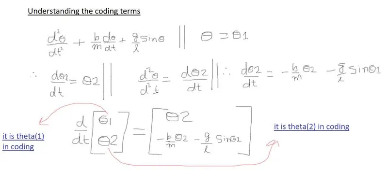
function [dtheta_dt] = challenge_func(t,theta,b,g,l,m) {name of function is "challenge_func" whose main inputs are t,theta,b,g,l,m & further it is stored in [dtheta_dt]}
theta1=theta(1); {theta1 is variable & theta is matrix thats why I have written theta(1) which is basically 1st value of column matrix & stored in theta1}
theta2=theta(2); {theta2 is variable & theta is matrix thats why I have written theta(2) which is basically 2nd value of column matrix & stored in theta2}
dtheta1_dt=theta2; {described in picture}
dtheta2_dt=((-b/m)*dtheta1_dt)-((g/l)*sin(theta1)); {it is also described in picture}
dtheta_dt=[dtheta1_dt;dtheta2_dt]; {here I have done both equation in matrix column and stored in column array}
end
"Please find link of my animation at end of the page"
% CODING
clear all
close all
clc

b=0.05; % damping co-efficient
g=9.81; % gravity
l=1; % length
m=1; % mass

% initial condition
theta_initial=[0;3];

% time points
time_duration=linspace(0,20,501);

% solution of ode in MATLAB
[t, results]=ode45(@(t,theta) challenge_func(t,theta,b,g,l,m),time_duration,theta_initial);

figure(1)
plot(t,results(:,1),"Color",'b','LineWidth',1.5)
hold on
plot(t,results(:,2),"Color",'r','LineWidth',1.5)
xlabel('Time in Seconds')
ylabel("Angular Displacement & Angular Velocity")
legend('Angular Displacement','Angular Velocity')


x=l*sin(results(:,1));
y=l*cos(results(:,1));

counter=1;
for Z=1:length(time_duration)
    X=x(Z);
    Y=-y(Z);
    x_initial=0;
    y_initial=0;

    figure(2)
    plot([x_initial X],[y_initial Y],'Marker',"o",'Color','b','linewidth',1,'MarkerFaceColor','y','MarkerSize',11)
    axis([-2 2 -2 2])
    pause(0.03)
    MV(counter)=getframe(gcf);
    counter=counter+1;

end

movie(MV);
vf=VideoWriter('Simple Pendulum.avi','Uncompressed AVI');
open(vf)
writeVideo(vf,MV)
close(vf)
% VIDEO LINK