Week 4.1 - Genetic Algorithm

Stalagmite function

function [stalagmite] = stalagmite_func(input_vector)

x= input_vector(1);

y = input_vector(2);

f1_x=(sin(5.1*pi* x +0.5)).^6;
f2_y = (sin(5.1*pi*y +0.5)).^6;
f3_x = exp((-4*0.6931).*(x-0.0667)^2/(0.64)); 
f4_y = exp((-4*0.6931).*(y-0.0667)^2/(0.64));

stalagmite=-(f1_x.*f2_y.*f3_x.*f4_y);

end

clear all
close all
clc

% PROVIDING THE SEARCH SPACE FOR THE FUNCTION

x=linspace(0,0.6,150);
y=linspace(0,0.6,150);
[X,Y]=meshgrid(x,y);
num_cases=50; %Number of itreation for which the function will evaluate the fitness

% Evaluvating the stalagmite function
for i=1:length(X)
for j=1:length(Y)
input_vector(1)=X(i,j);
input_vector(2)=Y(i,j);
f(i,j)=stalagmite_func(input_vector); %values of function in given search space
end
end

% STATISTICAL BEHAVIOUR (UNBOUNDED)

tic %calculating the study time through tic and toc command
for i=1:num_cases
[inputs,fopt(i)]=ga(@stalagmite_func,2); %calculating the optimized value of the function
xopt(i)=inputs(1); %at each iteration
yopt(i)=inputs(2);
end
study1_time=toc; %displaying the time taken to evaluate

% PLOTING THE GRAPH

figure(1)
subplot(2,1,1)
surfc(X,Y,-f);
hold on
shading interp
plot3(xopt,yopt,-fopt,'marker','o','markersize',5,'markerfacecolor','r');
xlabel('x');
ylabel('y');
grid on
subplot(2,1,2)
plot(-fopt);
xlabel('iterations')
ylabel( 'function max value')

% STATISTICAL BEHAVIOUR (BOUNDED)

tic %calculating the study time through tic and toc command
for j=1:num_cases
    [inputs,fopt(j)]=ga(@stalagmite_func,2,[],[],[],[],[0;0],[.6;0.6]); %calculating the optimized value of the function 
    xopt(j)=inputs(1); %at each iteration with boundation
    yopt(j)=inputs(2);
end
study2_time=toc;

%PLOTTING

figure(2)
subplot(2,1,1)
hold on
surfc(X,Y,-f)
shading interp
plot3(xopt,yopt,-fopt,'marker','o','markersize',5,'markerfacecolor','r');
xlabel('x');
ylabel('y');
grid on
subplot(2,1,2)
plot(-fopt);
xlabel('iterations')
ylabel('function max value')

% MODIFYING THE NUMBER OF POPULATION

options=optimoptions('ga','populationsize',300) %increaing the sixe of population by using optimoptions function
tic
for k=1:num_cases
[inputs,fopt(k)]=ga(@stalagmite_func,2,[],[],[],[],[0;0],[0.6;0.6],[],[],options);
xopt(k)=inputs(1);
yopt(k)=inputs(2);
end
study3_time=toc;

%PLOTTING

figure(3)
subplot(2,1,1)
hold on
surfc(X,Y,-f)
shading interp
plot3(xopt,yopt,-fopt,'marker','o','markersize',5,'markerfacecolor','r');
xlabel('x');
ylabel('y');
grid on
subplot(2,1,2)
plot(-fopt);
xlabel('iterations')
ylabel('function max value')

Explanation

First we initialise the value of x and y taking 150 values between the interval 0 and 0.6 and considered number of iteration as 50.

To plot 3D surface we take the 2d array of x and y using meshgrid command and store them in input_vector array.

For first study

We take no of iterations =num_spaces and we use the genetic algorithm function to calculate the maxima of the function . Store the result into xopt,yopt. By plting the surface of x,y,-f 3D plot is obtained. Then plotting it into the surf command and also providing the optimum values of the function that how it is varying. Also using the tic and tok command to evaluate the time used for optimizing the function.

for bounded values

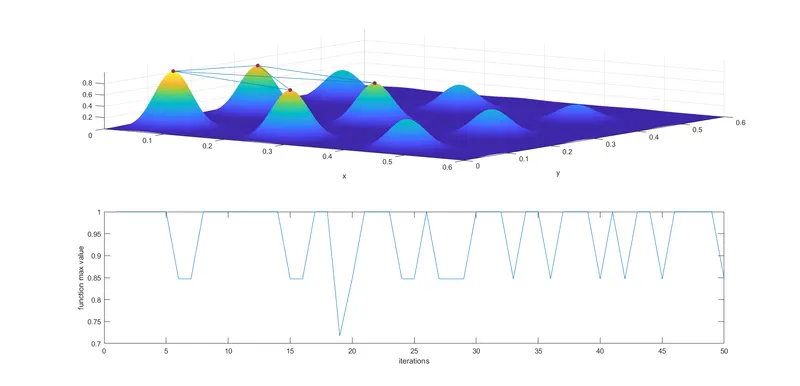
Store the result into xopt,yopt now we need to plot the surface of x,y,-f to get 3Dplot. plot3 command is used to make the plot of xopt,yopt and -fopt. tic and toc commands are used to get time taken to complete the cycle.

Increasing initial population

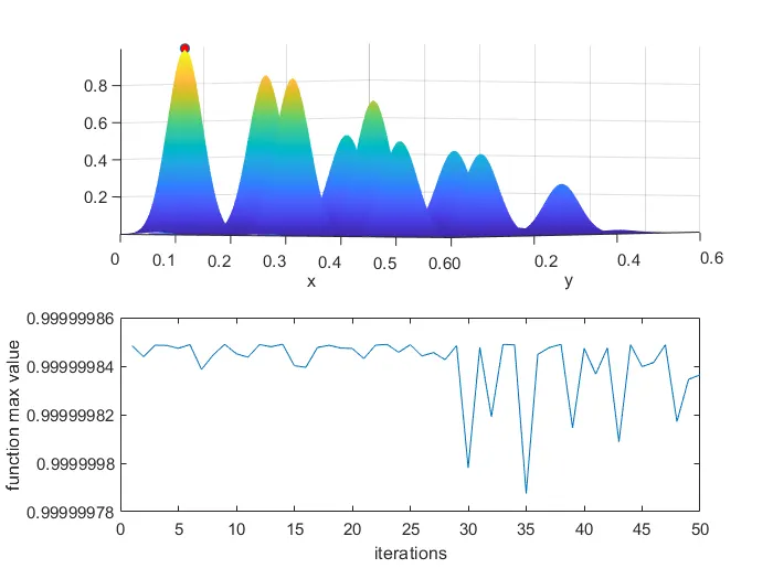
In this study using the ‘optimoptions’ command to increase the size of population.

all other commands are same as above.

Result

Unbounded condition

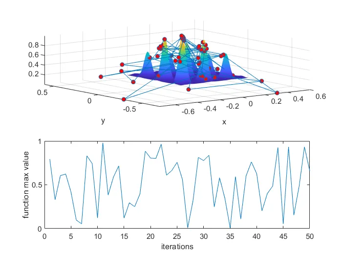
Here we can see the optimal values went outside the values of x and y resulting in falling away from stalagmite surface.

Bounded condition

Modifying number of population

Syntax for ga

x = ga(fun, nvars)

x = ga(fun, nvars, A,b)

x = ga(fun, nvars, A, b, Aeq, beq)

x = ga(fun, nvars, A, b, Aeq, beq, lb, ub)

x = ga(fun, nvars, A, b, Aeq, beq, lb, ub, nonlcon)

x = ga(fun,nvars, A, b, Aeq, beq, lb, ub, nonlcon, options)

x = ga(fun, nvars, A,b,[],[],lb, ub, nonlcon, IntCon)

x = ga(fun,nvars,A,b,[],[],1b, ub, nonlcon, IntCon, options) x = ga(problem)

[x, fval] = ga(_____)

[x, fval, exitflag, output] = ga(_____) [x, fval, exitflag,output, population, scores] = ga(_____)