Week 4.1 - Genetic Algorithm

Function representation of the stalagmite GA algoritham calculation

Explanation Ga function

X=ga(func,Nvars,A,B,Aeq,Beq,lb,ub,Nonlcon)

GA function representation

func-function name

Nvars-number of the variables

A,B-Matrix maltiplyers

Aeq,Beq- linear value

lb,ub-lower & upper boundaries

Nonlcon-n constant value of the

%Function method, What is the equation of the function,could be present

function [f]= stalagmite(input_vector)

%input vector equal to inputs

x=input_vector(1);
y=input_vector(2);

f1_x=(sin((5.1*pi*x)+0.5)).^6;
t1=((x-0.0667).^2/0.64);
f2_x=exp(-4.*log(2)*t1);
f1_y=(sin((5.1*pi*y)+0.5)).^6;
t2=((y-0.0667).^2/0.64);
f2_y=exp(-4.*log(2)*t2);
f= -(f1_x.*f1_y.*f2_x.*f2_y)
end

MAIN PROGRAME FOR GA CALCULATIONS

clear all;
close all;
clc;

%inputs of x,y
x=linspace(0,0.6,140);
y=linspace(0,0.6,140);
numcases=50;
[xx yy] = meshgrid(x,y)
grid on
for i=1:length(x)
for j=1:length( y)
input_vector(1)=xx(i,j);
input_vector(2)=yy(i,j);
f(i,j) = stalagmite(input_vector)%stalagmite function presented to calculating the function value
end
end
figure(1)
surfc(xx,yy,-f)

shading interp%remove the grid line from the figures

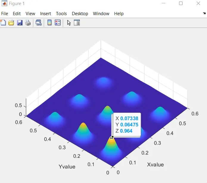
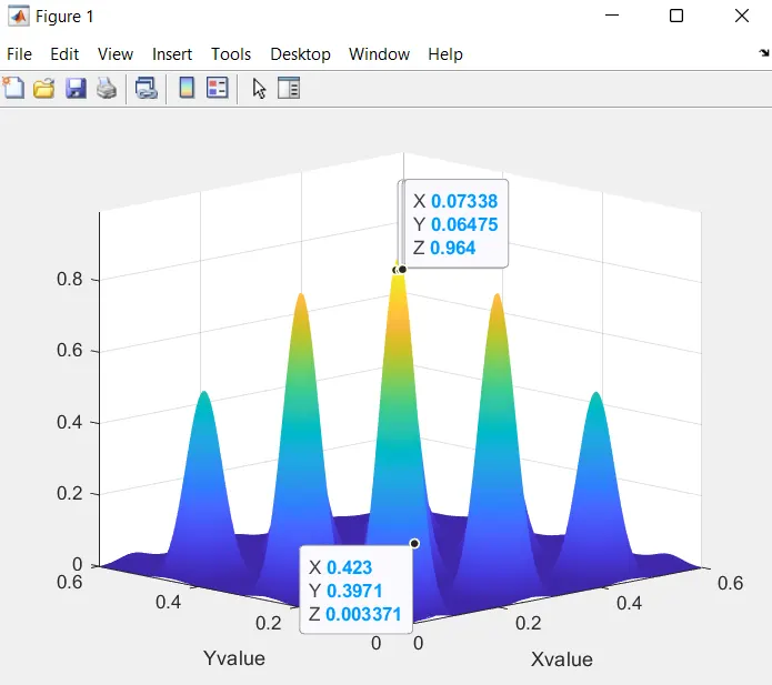
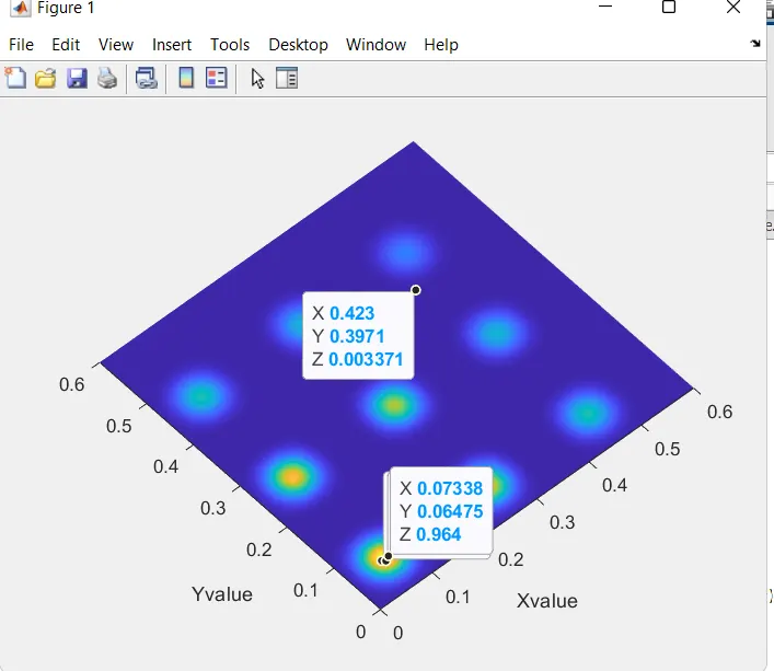
local maxima 0.964

% study statical behavior non standard
tic
for i=1:numcases;
[input,fopt1(i)]=ga(@stalagmite,2);%gA function representation
xvalue1(i)=input(1);
yvalue1(i)=input(2);
end

study1_time=toc
figure(2)
subplot(2,1,1)% create another plot in same images
surfc(x,y,-f);% Creating surface for the outputs
shading interp
hold on
plot3(xvalue1,yvalue1,-fopt1,'marker','o','markersize',5,'markerfacecolor','r')%markers for the local minima and maxima
xlabel('x')
ylabel('y')
title('Unbounded Results')
grid on
subplot(2,1,2)
plot(-fopt1)%plot othe outputs
xlabel('iteration')
ylabel('function min value')
title('unbounded Results')

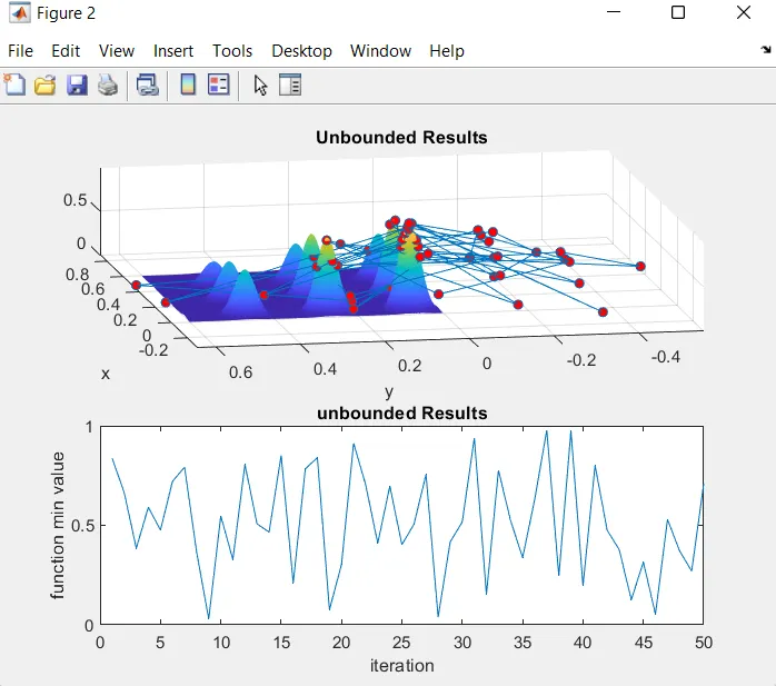
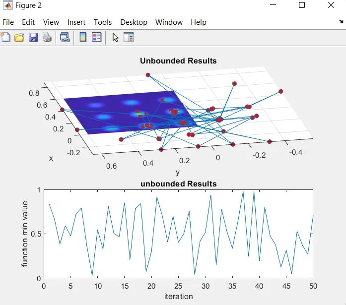
local maxima is 0.987

%study statical behavior standard
tic
for j=1:numcases;
[input,fopt2(j)]=ga(@stalagmite,2,[],[],[],[],[0;0],[1,1]);%ga function with boundaries
xvalue1(j)=input(1);
yvalue1(j)=input(2);
end
study2_time = toc
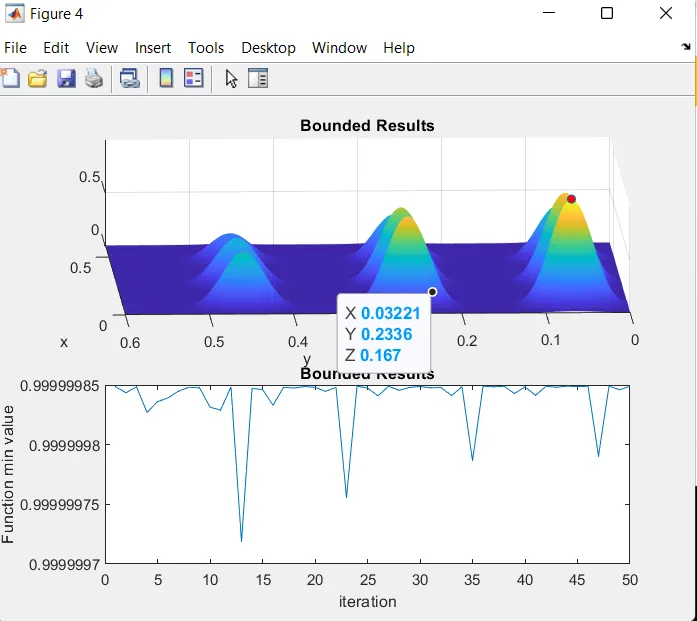
figure(3)
subplot(2,1,1)
surfc(x,y,-f)
shading interp
hold on
plot3(xvalue1,yvalue1,-fopt2,'marker','o','markersize',5,'markerfacecolor','r')
xlabel('x')
ylabel('y')
title('Bounded Results')
grid on
subplot(2,1,2)
plot(-fopt2)
xlabel('iteration')
ylabel('Function min value')
title('Bounded Results')

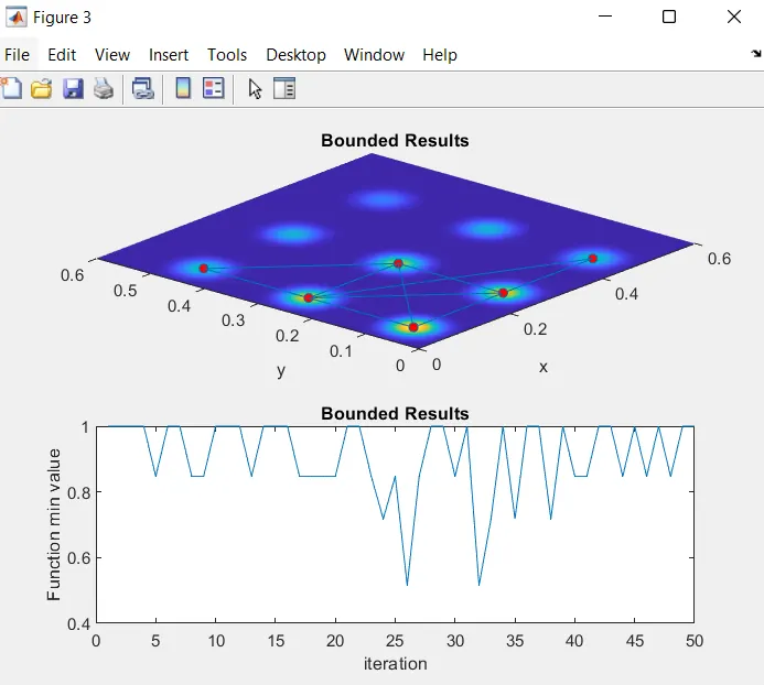
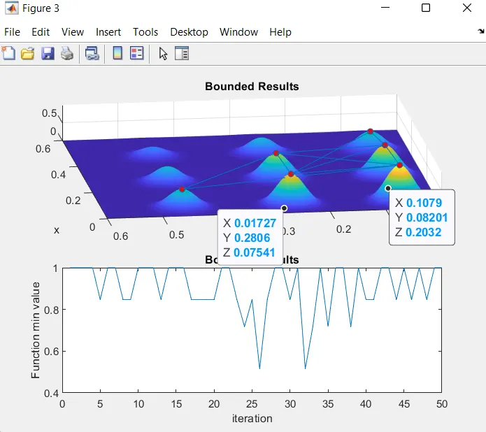
local maxima of this bounded study is 1

options=optimoptions('ga','populationsize',300)
for j=1:numcases;
[input,fopt3(j)]=ga(@stalagmite,2,[],[],[],[],[0;0],[1,1],[],[],options);
xvalue1(j)=input(1);
yvalue1(j)=input(2);
end
study3_time = toc
figure(3)
subplot(2,1,1)
surfc(x,y,-f)
shading interp
hold on
plot3(xvalue1,yvalue1,-fopt3,'marker','o','markersize',5,'markerfacecolor','r')
xlabel('x')
ylabel('y')
title('Bounded Results')
grid on
subplot(2,1,2)
plot(-fopt3)
xlabel('iteration')
ylabel('Function min value')
title('Bounded Results')

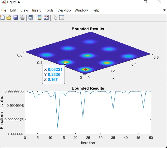
local maxima of this study 0.99999