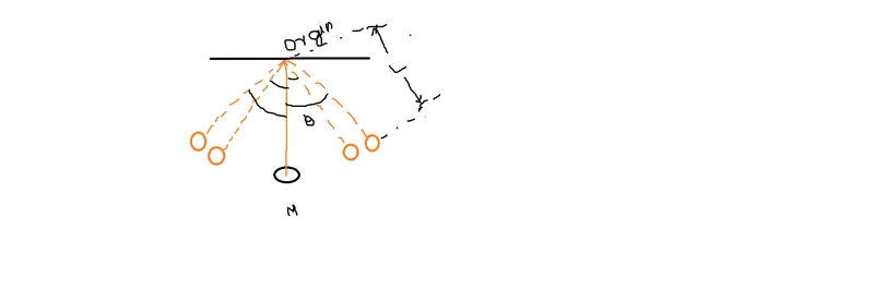
Week 3 - Solving second order ODEs

Ode solver equation, second oder eqaution

Important to solve methord of the equatin that are all, very important in matlab simulink coding

ode solver very important in the role of solve ode equation, Ode45, Ode23,Ode15 that are all the type of solvers,

seond oder bendulam equation two step to follow the method of solving

1.Function creation

2.main solver coding

Deferntial equation

dtheda1/dt=theda2, theda/dt=dthda1/dt; theda=theda1;

dtheda2/dt =dtheda1^2/dt^2;

Tittle of fun_ode Function calling

>that is going to be easy solution solving equation

function [theda_dt]=fun_ode(t,theda)
L=1;g=9.81;b=0.05;
m=1;
theda1=theda(1);
theda2=theda(2);
theda1_dt=theda2;
theda2_dt=(-b/m)*theda2-(g/L)*sin(theda1);
[theda_dt]=[theda2;theda2_dt];

end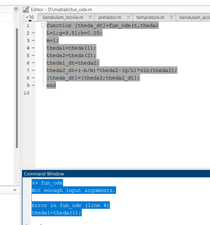

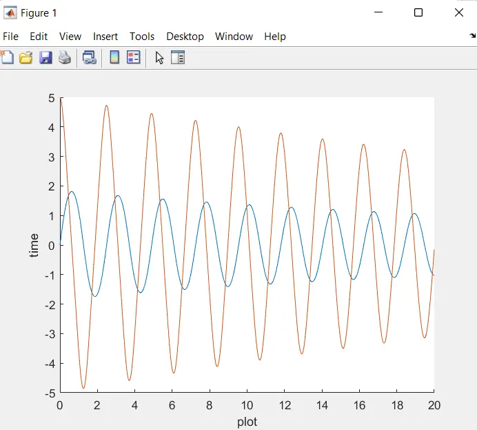
Noramal equation of the equation

close all,
clear all,clc

%input parameters
g=9.8;
b=0.05;
L=1;
m=1;

%respected angle
theda_0=[0; 5];
%t_span
t_span=linspace(0,20,500);
%ode derivation

[t,results]=ode45('fun_ode',t_span,theda_0)
figure(1)
hold on
plot(t,results(:,1))
plot(t,results(:,2))
xlabel('plot')
ylabel('time')

Main program for solving equation

close all,clear all,clc,

%input parameters for the length of the bendulam
L=1;
%Respected angle for bendulam displacement
theda_0=[0 5];
%t_span for bendulam ocilation movement
t_span=linspace(0,50,100);
%ode derivation solver function coresponted theda and t _span interval
[t,results]=ode45('fun_ode',t_span,theda_0);
figure(1)
hold on
plot(t,results(:,1),'linewidth',3)
plot(t,results(:,2),'linewidth',3)
xlabel('plot')
ylabel('time')

% Bendulam animation
%initial position bendulam tiighted in x axis orgin positon
X0=0;
Y0=0;

ct=1;

for i=1:length(t)
X1=L*sin(results(i,1));%Bendulam oscilation in x axis direction
Y1=-L*cos(results(i,1));%Bendulam oscilation in y axis direction
figure(2)
%bendulam coresponding limits
plot([-1 1],[0 0],'linewidth',2,'color','g');%bendulam support axis limit
axis([-2 2 -2 1]);
line([X0 X1],[Y0 Y1],'linewidth',1,'color','b');%bendulam length
hold on
% marking of the bendulam spilit outs
plot(X0,Y0,'O','markersize',5,'markerfacecolor','y');%bendulam tie location point
plot(X1,Y1,'O','markersize',20,'markerfacecolor','r');%ball of the bendulam
title('damping pendulam');
%Intication of every intividual part of the bendulam
legend('support rod','length of bendulam','Fixed point','board of bendulam');
grid on;
hold off;
pause(0.01);
M(ct)=getframe(gcf);
ct=ct+1;

end
movie(M)
videofile=VideoWriter('acilation.avi','uncompressed AVI');
open(videofile);
writeVideo(videofile,M);
close(videofile);

Final output of the program

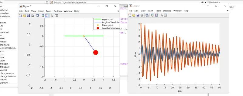
Bendulam explaination

length of the bendulam and mass that are all changing the dispalcemnt of the bendulam direction

Bendualm tie with Rod, Then the length of the Bendulamin X,Y direction movement displacement varied, that reprasents

X1=Lsin(Resulted (1,L))

Y1=-Lcos(Resulted (1,L))

Resulted value displacment of bendulam with respected to the time of the equation

Angular variation of value it gonig to be Resulted (1,L)

Every time it is varied resulted depend upon the time it is equal to angular value

Force of the bendulam changing depended value of gravity ,

gravity relation directly affected by the mass of the bendulam, the bendulam acilation going to be stop at the end, but the ocilation time of the bendulam varied