Week 4.1 - Genetic Algorithm

Aim : To write MATLAB code to optimise the stalagmite function and Global Maxima of the function.

Theory

Optimization is a process of finding desirable solution of a given problem which leads to the best performance under the give constraints. The genetic algorithm repeatedly modifies a population of individual solutions.

At each step, the genetic algorithm selects individuals. at random from the current population to be parents and uses them to produce the children for the next generation . Over successive generations, the population evolves toward an optimal solution.

You can apply the genetic algorithm to solve a variety of optimization problems that are not well suited for standard optimization algorithms, including problems in which the objective function is discontinuous, non- differentiable, stochastic or highly non-linear. The genetic algorithm can address problems of mixed- integer programming, where some components are restricted to be integer-valued.

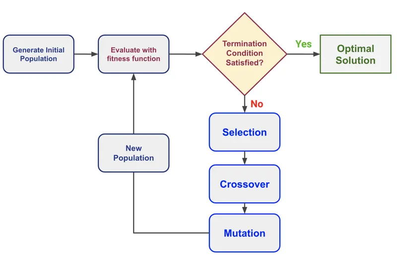
Phases in Genetic Algoritham-

1. Selection

The idea of the selection phase is to select the fittest individuals and let them pass their genes to the next generation. The main goal of this phase is to find the region where the chances of getting the best solution are more.

Inspiration for this is from the survival of the fittest.

It should be a balance between exploration and exploitation of search space.

GA tries to move the genotype to higher fitness in the search space.

Too strong fitness selection bias can lead to sub-optimal solutions.

Too little fitness bias selection results in unfocused search

2. Reproduction

Generation of offspring happen in 2 way:

Crossover

Mutation

3. Crossover

Crossover is the most significant stage in the genetic algorithm. During crossover, a random point is selected while mating a pair of parents to generate offspring.

There are 3 major types of crossover.

Single Point Crossover:

A point on both parents’ chromosomes is picked randomly, and designated a ‘crossover point’.

Two-Point Crossover: Two crossover points are picked randomly from the parent chromosomes.

Unifofm Crossover: In a uniform crossover, typically, each bit is chosen from either parent with equal probability.

4. Mutation

In a few new offspring formed, some of their genes can be subjected to a mutation with a low random probability. This indicates that some of the bits in the bit chromosome can be flipped. Mutation happens to take care of diversity among the population and stop premature convergence.

Stalagmite Function Code :

function[f]= stalagmite(input)
x = input(1);
y = input(2);

f1x =(sin(((5.1*pi).*x)+0.5)).^6;
f1y =(sin(((5.1*pi).*y)+0.5)).^6;

f2x = exp ((((x-0.0667).^2).*(-4*log(2)))./0.64); 
f2y = exp ((((y-0.0667).^2).*(-4*log(2)))./0.64); 

f=-f1x*f1y*f2x*f2y;

end

Code for Genetic Algorithm :

clear all
close all
clc
% search space
x=linspace(0,0.6,150);
y=linspace(0,0.6,150);
num_cases=50;

% two dimensional mesh 

[xx, yy] = meshgrid(x,y);

%evaluating the stalagmite function 
for i= 1:length(xx)
    for j = 1:length(yy)
        input(1)=xx(i,j);
        input(2)=yy(i,j);
        f(i,j)=stalagmite(input);
    end
end
% study 1 - statistical behaviour of genetic algorithm
tic

for i = 1: num_cases
   [inputs,fopt(i)]= ga(@stalagmite,2);
    xopt(i)= inputs(1);
    yopt(i)= inputs(2);
end
% 
fopt = -fopt
f=-f
study1_time =toc
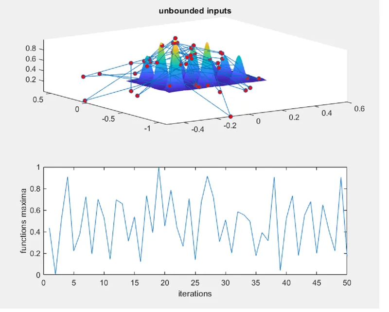
figure(1)
subplot(2,1,1)
hold on
surfc(x,y,f)
shading interp
plot3(xopt,yopt,fopt,'marker','o','markersize',5,'markerfacecolor','r')
title('unbounded inputs')
subplot(2,1,2)
plot(fopt)
xlabel('iterations')
ylabel('functions maxima')

%study 2 - statistical behaviour with upper and lower bounds
tic
for i = 1: num_cases
   [inputs,fopt(i)]= ga(@stalagmite,2,[],[],[],[],[0:0],[1:1]);
   xopt(i)= inputs(1);
   yopt(i)= inputs(2);
end
fopt=-fopt
f=-f

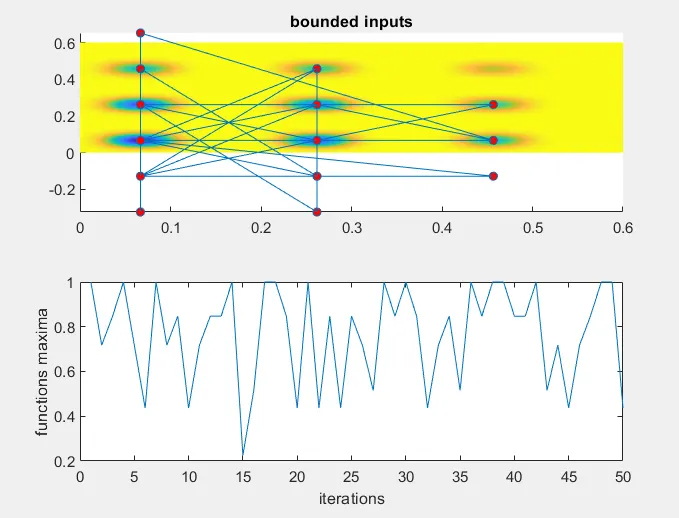
figure(2)
subplot(2,1,1)
hold on
surfc(x,y,f)
shading interp
plot3(xopt, yopt,fopt, 'marker','o','markersize',5,'markerfacecolor','r')
title('bounded inputs')
subplot(2,1,2)
plot(fopt)
xlabel('iterations')
ylabel('functions maxima')

% study 3 increasing GA iteration 
options = optimoptions('ga');
options = optimoptions(options, 'populationsize',500);
tic
for i = 1:num_cases
 [inputs,fopt(i)]= ga(@stalagmite,2,[],[],[],[],[0:0],[1:1],[],[],options);
 xopt(i)= inputs(1);
 yopt(i)= inputs(2);
end
fopt=-fopt
f=-f

study3_time =toc

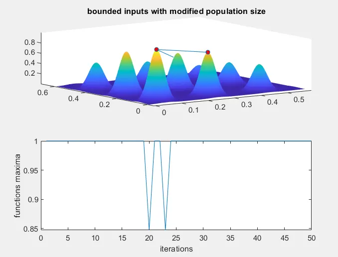
figure(3)
subplot(2,1,1)
hold on
surfc(x,y,f)
shading interp

plot3(xopt, yopt,fopt, 'marker','o','markersize',5,'markerfacecolor','r')
title('bounded inputs with modified population size')
subplot(2,1,2)
plot(fopt)
xlabel('iterations')
ylabel('functions maxima')

Results: