Week 3 - Solving second order ODEs

Aim :

Write a program that solves the following ODE. This ODE represents the equation of motion of a simple pendulum with damping.

Theory:

Definition

In mathematics, the term “Ordinary Differential Equations” also known as ODE is an equation that contains only one independent variable and one or more of its derivatives with respect to the variable. In other words, the ODE is represented as the relation having one independent variable x, the real dependent variable y, with some of its derivatives.

y’,y”, ….yⁿ ,…with respect to x.

Order

The order of ordinary differential equations is defined to be the order of the highest derivative that occurs in the equation. The general form of n-th order ODE is given as;

F(x, y,y’,….,yⁿ ) = 0

Note that, y’ can be either dy/dx or dy/dt and yⁿ can be either dⁿy/dxⁿ or dⁿy/dtⁿ.

An n-th order ordinary differential equations is linear if it can be written in the form;

a₀(x)yⁿ + a₁(x)y^n-1 +…..+ a_n(x)y = r(x)

The function a_j(x), 0 ≤ j ≤ n are called the coefficients of the linear equation. The equation is said to be homogeneous if r(x) = 0. If r(x)≠0, it is said to be a non- homogeneous equation. Also, learn the first-order differential equation here.

Types

The ordinary differential equation is further classified into three types. They are:

• Autonomous ODE
• Linear ODE
• Non-linear ODE

Autonomous Ordinary Differential Equations

A differential equation which does not depend on the variable, say x is known as an autonomous differential equation.

Linear Ordinary Differential Equations

If differential equations can be written as the linear combinations of the derivatives of y, then they are called linear ordinary differential equations. These can be further classified into two types:

• Homogeneous linear differential equations
• Non-homogeneous linear differential equations

Non-linear Ordinary Differential Equations:

If the differential equations cannot be written in the form of linear combinations of the derivatives of y, then it is known as a non-linear ordinary differential equation.

Applications:

ODEs has remarkable applications and it has the ability to predict the world around us. It is used in a variety of disciplines like biology, economics, physics, chemistry and engineering. It helps to predict the exponential growth and decay, population and species growth. Some of the uses of ODEs are:

• Modelling the growth of diseases
• Describes the movement of electricity
• Describes the motion of the pendulum, waves
• Used in Newton’s second law of motion and Law of cooling

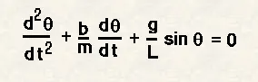
use,

L=1 metre,

m=1 kg,

b=0.05.

g=9.81 m/s2.

clc
clear all
close all

b= 0.05;
g= 9.81;
l= 1;
m= 1;

% intial condition 

theta= [0;3];
%time points 
t_span = linspace(0,20,500);
% solve ode 
[t,results]= ode45(@(t,theta)ode_func(t,theta,b,g,l,m),t_span,theta);

plot(t,results(:,1))
ylabel('plot');
xlabel('time');

ct=1;
 for i = 1: length(results(:,1))
     x0=0;
     y0=0;
     x1=l*sin(results(i,1));
     y1=-l*cos(results(i,1));
     plot([0,0],[1,1],'LineWidth',4,'Color','k');
     hold on
     plot(x1,y1,'o');
     plot([x0,x1],[y0,y1]);
     grid on;
     axis([-1.5 1.5 -1.5 0.5]);
     pause(0.0003);
     hold off;
     q(ct)=getframe(gcf);
     ct=ct+1;
 end
 figure(2)
 movie(q)
 videofile = VideoWriter('c:\matlab programs.m\pendulum.avi');
 open(videofile)
 writeVideo(videofile,q)
 close(videofile)

code Explaination :

Put all the give values in the give equation

plot the results

in for loop generate the x0, y0, x1, y1 values and plot those values on graph

used hold on cammand to observe the obtained results and used pause cammand for providing delay in the results obtained.

record the obtained results by movie command and save the animation video.

You Tube Link : https://youtu.be/L9-jSU625RQ

Conclusion :

We can solve any kind of ODE equation with help of this functions and obtained the results for further analysis.