Week 4.1 - Genetic Algorithm
Questions:
Try to understand the concept of genetic algorithm by referring to varius sources before you attend this challenge. Look out for information regarding stalagmite function and ways to optimise it.
- Write a code in MATLAB to optimise the stalagmite function and find the global maxima of the function.
- Clearly expalin the concept of genetic algorithm in your own words and also explain the syntax for ga in MATLAB in your report.
- Make sure that your code gives the same output, even if it is made to run several times.
- Plot graphs for all 3 studies and for F maximum vs no. of iterations. Title and axes labels are a must, legends could be shown if necessary.
Solution:
Definition: A Generic Algorithm is a optimization method for solving both constrained and unconstrained optimization problems based on natural selection process that mimics biological evolution techniques. It is also used to find global minima for highly nonlinear problems.
|
Classical Algorithm |
Genetic Algorithm |
|
Generates a single point at each iteration. The sequence of points approaches an optimal solution. |
Generates a population of points at each iteration. The best point in the population approaches an optimal solution. |
|
Selects the next point in the sequence by a deterministic computation. |
Selects the next population by computation which uses random number generators. |
Benefits of Optimization
- Finding better(optimal) designs
- Faster design evaluations
- Useful for trade-off analysis
- Non-intuitive designs may be found
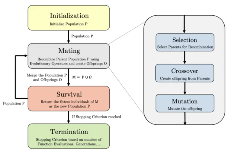
Description of the above flow chart: A genetic algorithm starts with initializing individuals forming the population P of a predefined size |P|. The population P undergoes the process of mating, which has the goal of producing offspring O through recombination. To generate offspring through mating, the population must go through parental selection, crossover, and mutation. Then, the population P and offspring O are merged to the solution set M of size |P+O|. The survival reduces M again to a solution set of size |P| by selecting only the fittest individuals. The resulting truncated population is then used for recombination in the next generation. This process is repeated until the termination criterion is met.
- Evaluate: The actual problem to be solved, where the function determines the fitness of each individual.
- Initialize: This method returns the initial population P.
- Selection: A function returning the individuals in the population functioning as parents for recombination.
- Crossover: A function creating one or multiple offspring given two or more parents.
- Mutation: A method mutation each offspring with a specific probability.
- Survival: A function reducing the merged population to a set of solutions equal to the population size by applying the principle of survival of the fittest.
Sometimes, the goal of an optimization is to find the global minimum or maximum of a function – a point where the function value is smaller or larger at any other point in the search space.
"ga" Syntax and description:
Syntax 1:
x = ga(fun,nvars)
x = ga(fun,nvars) finds a local unconstrained minimum, x, to the objective function, fun. nvars is the dimension (number of design variables) of fun.
Syntax 2:
x = ga(fun,nvars,A,b)
x = ga(fun,nvars,A,b) finds a local minimum x to fun, subject to the linear inequalities A*x ≤ b. ga evaluates the matrix product A*x as if x is transposed (A*x').
Syntax 3:
x = ga(fun,nvars,A,b,Aeq,beq)
x = ga(fun,nvars,A,b,Aeq,beq) finds a local minimum x to fun, subject to the linear equalities Aeq*x = beq and A*x ≤ b. (Set A=[] and b=[] if no linear inequalities exist.) ga evaluates the matrix product Aeq*x as if x is transposed (Aeq*x').
Syntax 4:
x = ga(fun,nvars,A,b,Aeq,beq,lb,ub)
x = ga(fun,nvars,A,b,Aeq,beq,lb,ub) defines a set of lower and upper bounds on the design variables, x, so that a solution is found in the range lb ≤ x ≤ ub. (Set Aeq=[] and beq=[] if no linear equalities exist.)
Syntax 5:
x = ga(fun,nvars,A,b,Aeq,beq,lb,ub,nonlcon)
x = ga(fun,nvars,A,b,Aeq,beq,lb,ub,nonlcon) subjects the minimization to the constraints defined in nonlcon. The function nonlcon accepts x and returns vectors C and Ceq, representing the nonlinear inequalities and equalities respectively. ga minimizes the fun such that C(x) ≤ 0 and Ceq(x) = 0. (Set lb=[] and ub=[] if no bounds exist.)
Syntax 6:
x = ga(fun,nvars,A,b,Aeq,beq,lb,ub,nonlcon,options)
x = ga(fun,nvars,A,b,Aeq,beq,lb,ub,nonlcon,options) minimizes with the default optimization parameters replaced by values in options. (Set nonlcon=[] if no nonlinear constraints exist.) Create options using optimoptions.
Syntax 7 & 8:
x = ga(fun,nvars,A,b,Aeq,beq,lb,ub,nonlcon,intcon)
x = ga(fun,nvars,A,b,Aeq,beq,lb,ub,nonlcon,intcon,options)
x = ga(fun,nvars,A,b,Aeq,beq,lb,ub,nonlcon,intcon) or x = ga(fun,nvars,A,b,Aeq,beq,lb,ub,nonlcon,intcon,options) requires that the variables listed in intcon take integer values.
Syntax 9:
x = ga(problem)
x = ga(problem) finds the minimum for problem, a structure described in problem.
Syntax 10:
[x,fval] = ga(___)
[x,fval] = ga(___), for any previous input arguments, also returns fval, the value of the fitness function at x.
Syntax 11:
[x,fval,exitflag,output] = ga(___)
[x,fval,exitflag,output] = ga(___) also returns exitflag, an integer identifying the reason the algorithm terminated, and output, a structure that contains output from each generation and other information about the performance of the algorithm.
Syntax 12:
[x,fval,exitflag,output,population,scores] = ga(___)
[x,fval,exitflag,output,population,scores] = ga(___) also returns a matrix population, whose rows are the final population, and a vector scores, the scores of the final population. 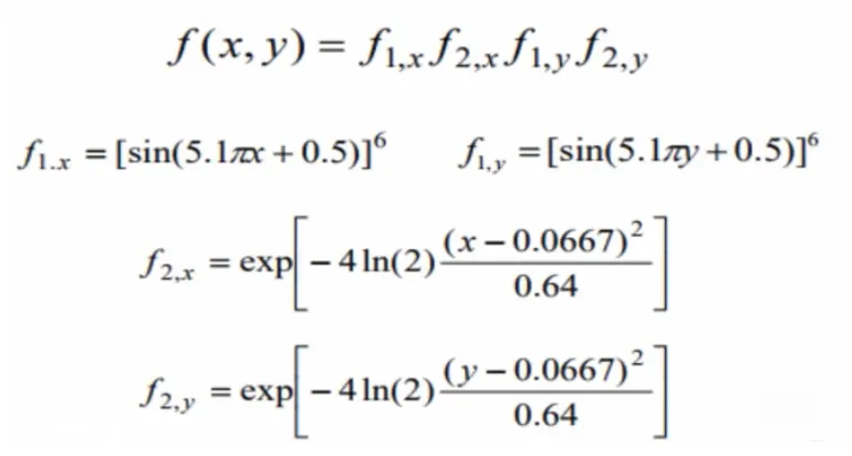
function [f] = stalagmite(input_vector)
x=input_vector(1);
y=input_vector(2);

f_1x=(sin(5.1*pi*x+0.5)).^6;
f_1y=(sin(5.1*pi*y+0.5)).^6;

f_2x=exp(-4.*log(2)*((x-0.0667).^2)./0.64);
f_2y=exp(-4.*log(2)*((y-0.0667).^2)./0.64);

f=-(f_1x.*f_2x.*f_1y.*f_2y);
end
Program Description:
Step 1: %cleaning command script- close all will closes all open MATLAB figure window, clear all will clear all data stored to a variable and the command clc will clear the command window.
Step2: linspace command is used to generate linearly spaced vector by generating 150 points and the spacing between the points is (0.6-0)/(150-1) which returns values for x and y variables.
Step 3: Meshgrid will create 2D and 3D grids. The below command will return 2-D grid coordinates based in the coordinates contained in vectors x and y. The grid is represented by the coordinates x and y has length(y) rows and length(x) columns.
Step 4: Evaluating the stalagmite function and plotting the figure with surface plot command. Below surface plot command will create a 3 Dimensional surface plot, which is a three-dimensional surface that has solid edge colors and solid face colors.Figure command is used to generate the plot with xlabel and ylabel to provide labels to the graphical representation of x-axis and y-axis. Shading interep will control the color shading of the surface and patch graphical objects. Shading Interp varies the color in each line segment and face by interpolating the colormap index or true color value across the line or face.
%cleaning
clear all
close all
clc

%Defining our search space or one dimensional
x = linspace(0,0.6,150)
y = linspace(0,0.6,150)

%creating a 2Dimensional mesh
[xx,yy]=meshgrid(x,y)

%Evaluating the stalagmite function
for i=1:length(xx)
    for j = 1:length(yy)
        input_vector(1)=xx(i,j);
        input_vector(2)=yy(i,j);
        f(i,j)=stalagmite(input_vector);
    end
end
figure(1)
surfc(xx,yy,-f)%to create surface plot
shading interp %controls shading of surface and patch graphics objects
[inputs, fval]=ga(@stalagmite,2)
xlabel('Values of x') %x-axis label
ylabel('Values of y') %y-axis label
title('General Stalagmite model')
Output: Global Maxima 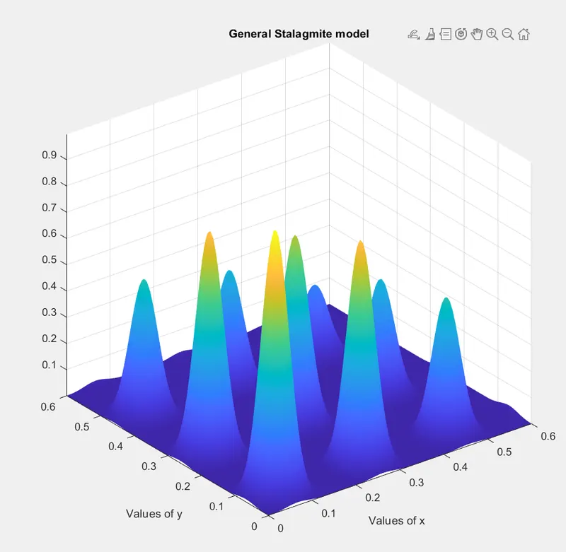
Case 2: Study without Boundation:
Function get_stalagmite:
This function is used for below three cases:
function [f] = get_stalagmite(x,y)

f_1x=(sin(5.1*pi.*x+0.5)).^6;
f_1y=(sin(5.1*pi*y+0.5)).^6;

f_2x=exp(-4.*log(2)*((x-0.0667).^2)./0.64);
f_2y=exp(-4.*log(2)*((y-0.0667).^2)./0.64);

f=-(f_1x.*f_2x.*f_1y.*f_2y);
end
Step 1: %cleaning command script- close all will closes all open MATLAB figure window, clear all will clear all data stored to a variable and the command clc will clear the command window.
Step2: linspace command is used to generate linearly spaced vector by generating 150 points and the spacing between the points is (0.6-0)/(150-1) which returns values for x and y variables.
Step 3: Tic and toc command were used to measure the time taken to perform the iterations input provided to the function and to generate the plots.
Step 4: num_cases= 50 performs 50 iterations and [inputs,fopt(i)] will be storing the optimal output by using the genetic algorithm solver. Subplot command will divide the current figure into rectabgular panes that are numbered row-wise.
Step 5: Meshgrid will create 2D and 3D grids. The below command will return 2-D grid coordinates based in the coordinates contained in vectors x and y. The grid is represented by the coordinates x and y has length(y) rows and length(x) columns. Plot 3 commands plots coordinates in 3D space.
%cleaning
clear all
close all
clc

%Defining our search space or one dimensional
x = linspace(0,0.6,150)
y = linspace(0,0.6,150)
%Giving number of iterations
[x,y]=meshgrid(x,y)
num_cases=50; %value of iterations
f = get_stalagmite(x,y) %to generate the stalagmite function
tic %calculating the study time
%Evaluating the stalagmite function
for i=1:num_cases
    [inputs, fopt(i)]=ga(@stalagmite,2) %storing
    xopt(i)=inputs(1);
    yopt(i)=inputs(2);
end
study1_time=toc %to display the time taken

%plotting
figure(1)
subplot(2,1,1) %to have multiple plots
surfc(x,y,-f)
hold on
shading interp
plot3(xopt,yopt,-fopt,'marker','o','MarkerSize',5,'MarkerFaceColor','r');
xlabel('Values of x') %giving x axis label
ylabel('Values of y') %giving y axis label
title('Unbounded inputs')
subplot(2,1,2)
plot(-fopt);
xlabel('iterations')
ylabel('function min value')
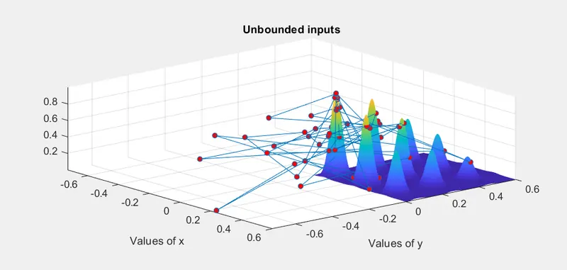
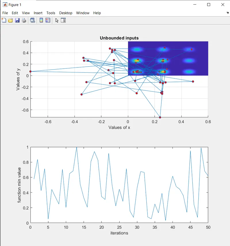
Output: Results obtained are not really helpful in evaluating the required output. It can be observed that there is a lot of variations with the represented red circular dots.
Case 3: Statistical study with upper and lower bounds
In this study, the stalagmite function is given upper and lower bounds of (0;0) and (1;1).
Tic and toc command were used to measure the time taken to perform the iterations input provided to the function and to generate the plots.
Meshgrid will create 2D and 3D grids. The below command will return 2-D grid coordinates based in the coordinates contained in vectors x and y. The grid is represented by the coordinates x and y has length(y) rows and length(x) columns. Plot 3 commands plots coordinates in 3D space.
%cleaning
clear all
close all
clc

%Defining our search space or one dimensional
x = linspace(0,0.6,150)
y = linspace(0,0.6,150)
%Giving number of iterations
[x,y]=meshgrid(x,y)
num_cases=50; %value of iterations
f = get_stalagmite(x,y) %to generate the stalagmite function
tic %calculating the study time
%Evaluating the stalagmite function
for i=1:num_cases
    [inputs, fopt(i)]=ga(@stalagmite,2,[],[],[],[],[0;0],[1;1]) %storing
    xopt(i)=inputs(1);
    yopt(i)=inputs(2);
end
study1_time=toc %to display the time taken

%plotting
figure(1)
subplot(2,1,1) %to have multiple plots
surfc(x,y,-f)
hold on
shading interp
plot3(xopt,yopt,-fopt,'marker','o','MarkerSize',5,'MarkerFaceColor','r');
xlabel('Values of x') %giving x axis label
ylabel('Values of y') %giving y axis label
title('Bounded inputs')
subplot(2,1,2)
plot(-fopt);
xlabel('iterations')
ylabel('function min value')
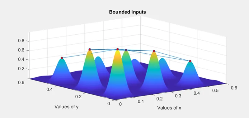
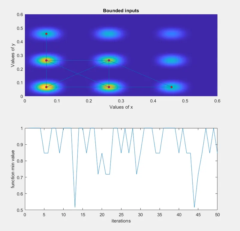
Output: The large variations is now limited by providing upper and lower bounds to the stalagmite function.
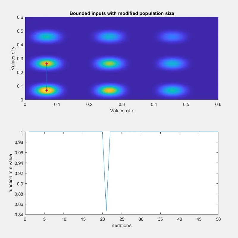
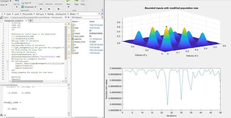
Case 4: Study with modified population size
Please refer to the below program included in population of size 400. The only change made is with respect to the below command:
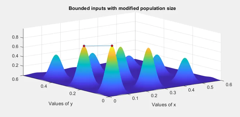
Population size to 200:Variation is compartively less to the variations obtained in previous cases.
Changing the population size to 400
Tic and toc command were used to measure the time taken to perform the iterations input provided to the function and to generate the plots.
Meshgrid will create 2D and 3D grids. The below command will return 2-D grid coordinates based in the coordinates contained in vectors x and y. The grid is represented by the coordinates x and y has length(y) rows and length(x) columns. Plot 3 commands plots coordinates in 3D space. Optimoptions was used to create optimization.
Syntax:
options = optimoptions(SolverName) returns a set of default options for the SolverName solver.
options = optimoptions(SolverName,Name,Value) returns options with specified parameters set using one or more name-value pair arguments.
%cleaning
clear all
close all
clc

%Defining our search space or one dimensional
x = linspace(0,0.6,150)
y = linspace(0,0.6,150)
%Giving number of iterations
[x,y]=meshgrid(x,y)
num_cases=50; %value of iterations
f = get_stalagmite(x,y) %to generate the stalagmite function
tic %calculating the study time
%increasing GA iterations
options=optimoptions('ga')
options=optimoptions(options,'PopulationSize',400)
%Evaluating the stalagmite function
for i=1:num_cases
    [inputs, fopt(i)]=ga(@stalagmite,2,[],[],[],[],[0;0],[1;1],[],[],options) %storing
    xopt(i)=inputs(1);
    yopt(i)=inputs(2);
end
study1_time=toc %to display the time taken

%plotting
figure(1)
subplot(2,1,1) %to have multiple plots
surfc(x,y,-f)
hold on
shading interp
plot3(xopt,yopt,-fopt,'marker','o','MarkerSize',5,'MarkerFaceColor','r');
xlabel('Values of x') %giving x axis label
ylabel('Values of y') %giving y axis label
title('Bounded inputs with modified population size')
subplot(2,1,2)
plot(-fopt);
xlabel('iterations')
ylabel('function min value')
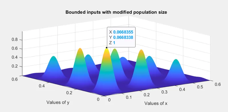
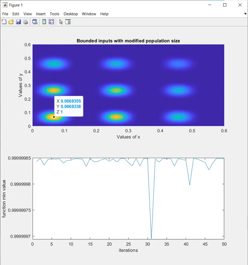
Output: The only disadvantage of this method is the study time to evaluate the stalagmite function due to the increase in the population size. But with this method the exact value of local maxima can be determined with better fitness and less variations as shown below in the graphical representation.
Errors Obtained:
Typo error: num_cases was not initialized for the loop to be executed for a given function.
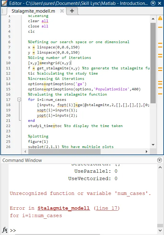
Rectification: Included num_cases = 50 to include the iteration value which further executed the plot output.
References:
Link to Generic Algorithm description:
https://in.mathworks.com/discovery/genetic-algorithm.html
Syntax for ga
https://in.mathworks.com/help/gads/ga.html
Optimoptions
https://in.mathworks.com/help/optim/ug/optim.problemdef.optimizationproblem.optimoptions.html
Genetic Algorithm