Week 4.1 - Genetic Algorithm

Genetic Algorithm

Developed by Prof. John holland, his colleagues at University of Michigan 1975.

1.Non traditional optimization technique.

2. Search algorithm based on the mechanics of natural selection and natural genetics.

3. Based on the 'survival of the fittest' concept.

4.simulated the process of evaluation.

5. Evolution is an optimizing process.

6.Ga work with the coding of the parameter set, not the parameters themselves, it looks for global minima.

7.Ga's search for a population of points, not a single point.

8.Ga's use objective function information and not the derivative or second derivative.

9.Ga's use stochastic transtion rules, not deterministic rules.

10. A polulation of 2n to 4n trail solutions is used (n is number of variables).

11.Each solution usually represented by a string of binary variables,corresponding to the chromosomes in genetics.

12.The string length can be made large enough to achieve any desired fitness of approximation and thus any desired accuracy can be achieved.

13.The numerical value of objective function corresponds to the concept of fitness in genetics.

14.After trail solutions are selected, a new generation( a new set of string) is produced by selecting, using probablistic principles, the fittest parents to produce"children" from among the trail solutions.

15. In each 'child' crossover or exchange of portion of string of each of thetwo parents generates new solution.

"The goal of optimizaion is keep improving performance to reach a or some optimal points."

Syntax for Genetic Algorithm

1. x= ga(fun,nvars)- finds local unconstrained minimum ,x, to the objective function, fun.nvars is the dimension of the fun.
2. x= ga(fun,nvars,A,b,Aeq,beq)-finds local minimum x to the function , A,b linear inequality constraint & Aeq,beq are linear equality constraint, if there are no linear equalities and inequalities then A,b ,Aeq,beq are set to [].
3. x=ga(fun,nvars,A,b,Aeq,beq,nonlcon,intcon,options) where nonlcon is non linear constraints, intcon is integer values and options is optimization options.

STALAGMITE FUNCTION:-

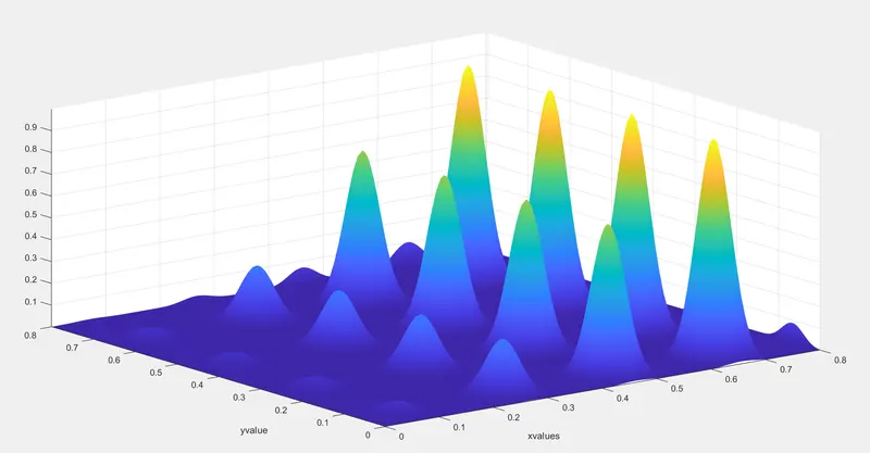
A stalagmite function generally refers to the function with which we are generating valuesover a stalagmite kind of surface for finding out the local and global maxima and minima of that particular function. For this in matlab we use a method called "optimization"

Now we are defining our objective function f as below:-

%define stalagmite function

function f=stalagmite(input_vector)

x=input_vector(1);

y=input_vector(2);

t1=(sin((5.1*pi*x)+0.5))^6;

t2=(sin((5.1*pi*y)+0.5))^6;

t3=exp(-4*log(2)*((x-0.667)^2)/0.64);

t4=exp(-4*log(2)*((x-0.667)^2)/0.64);

f=-(t1*t2*t3*t4);

end

Ga code case study 1

%define our search space

x=linspace(0,0.8,150);

y=linspace(0,0.8,150);

n=50;

%creating a 2D mesh

[xx, yy]=meshgrid(x,y);

%evaluating the stalagmite function

for i=1:length(xx)

for j=1:length(yy)

input_vector(1)=xx(i,j);

input_vector(2)=yy(i,j);

f(i,j)=stalagmite(input_vector);

end

end

surfc(xx,yy,f);

xlabel('xvalues')

ylabel('yvalue')

shading interp

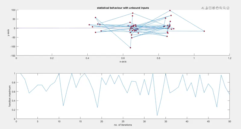
%study1 statistical behaviour

tic

for i=1:n

[inputs,fopt(i)]=ga(@stalagmite,2);

xopt(i)=inputs(1);

yopt(i)=inputs(2);

end

study1_time=toc;

figure(1)

subplot(2,1,1)

hold on

surf(xx,yy,-f)

shading interp

xlabel('x-axis');

ylabel('y-axis');

title ('statistical behaviour with unbound inputs');

plot3(xopt,yopt,-fopt,'marker','o','MarkerSize',5,MarkerfaceColor='r');

subplot(2,1,2)

plot(-fopt);

xlabel('no. of iterations')

ylabel('function maximum')

Ga code case study 2

%define our search space

x=linspace(0,0.8,150);

y=linspace(0,0.8,150);

n=50;

%creating a 2D mesh

[xx, yy]=meshgrid(x,y);

%evaluating the stalagmite function

for i=1:length(xx)

for j=1:length(yy)

input_vector(1)=xx(i,j);

input_vector(2)=yy(i,j);

f(i,j)=stalagmite(input_vector);

end

end

surfc(xx,yy,f);

xlabel('xvalues')

ylabel('yvalue')

shading interp

%study2 statistical behaviour

tic

for i=1:n

[inputs,fopt(i)]=ga(@stalagmite,2,[],[],[],[],[0;0],[1;1]);

xopt(i)=inputs(1);

yopt(i)=inputs(2);

end

study2_time=toc;

figure(1)

subplot(2,1,1)

hold on

surf(xx,yy,-f)

shading interp

xlabel('x-axis');

ylabel('y-axis');

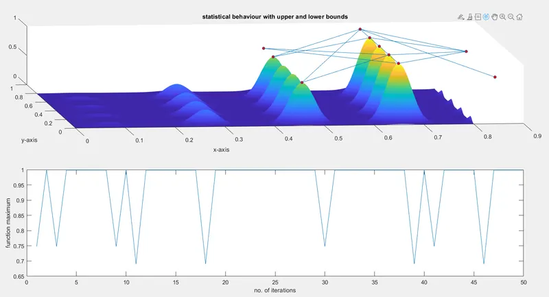
title ('statistical behaviour with upper and lower bounds');

plot3(xopt,yopt,-fopt,'marker','o','MarkerSize',5,MarkerfaceColor='r');

subplot(2,1,2)

plot(-fopt);

xlabel('no. of iterations')

ylabel('function maximum')

Ga code case study 3

%define our search space

x=linspace(0,0.8,150);

y=linspace(0,0.8,150);

n=50;

%creating a 2D mesh

[xx, yy]=meshgrid(x,y);

%evaluating the stalagmite function

for i=1:length(xx)

for j=1:length(yy)

input_vector(1)=xx(i,j);

input_vector(2)=yy(i,j);

f(i,j)=stalagmite(input_vector);

end

end

surfc(xx,yy,f);

xlabel('xvalues')

ylabel('yvalue')

shading interp

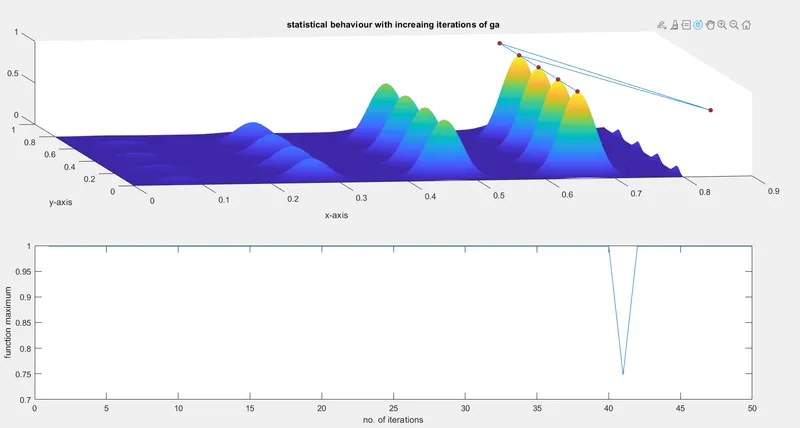
%study3 statistical behaviour with increasing iteraions of Ga

options=optimoptions('ga');

options=optimoptions(options,'populationsize',180);

tic

for i=1:n

[inputs,fopt(i)]=ga(@stalagmite,2,[],[],[],[],[0;0],[1;1],[],[],options);

xopt(i)=inputs(1);

yopt(i)=inputs(2);

end

study2_time=toc;

figure(3)

subplot(2,1,1)

hold on

surf(xx,yy,-f)

shading interp

xlabel('x-axis');

ylabel('y-axis');

title ('statistical behaviour with increaing iterations of ga');

plot3(xopt,yopt,-fopt,'marker','o','MarkerSize',5,MarkerfaceColor='r');

subplot(2,1,2)

plot(-fopt);

xlabel('no. of iterations')

ylabel('function maximum')