Week 4.1 - Genetic Algorithm

Code to optimise the stalagmite function :- We are using genetic algorithm to optimise the stalagmite function and we will get the minimum value of the optimised function because "GA" is only used to get the minimum value.

clear all;
close all;
clc;

% Defining the search space 
x=linspace(0,0.6,150);
y=linspace(0,0.6,150);

% creating the 2 D array / Mesh 
[xx yy] = meshgrid(x,y);

%Evaluating the stalagmite function 

for i=1:length(xx)
    for j=1:length(yy)
        input_vector(1)=xx(i,j);
        input_vector(2)=yy(i,j);
        f(i,j) = stalagmite(input_vector);
    end
end

surfc(xx,yy,f)
shading interp
[x,fval]=ga(@stalagmite,2);
title('Stalagmite function optimisation');
xlabel('x value');
ylabel('y value');

Plot :-

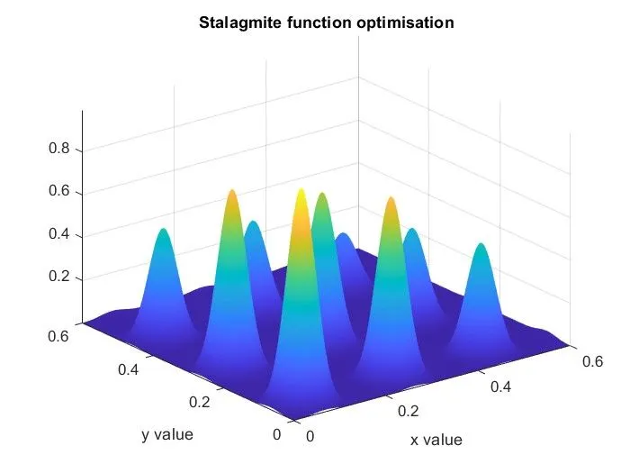
Explaination of the code :-

1. in the first three lines commands are used for clearing the workspace , closing all the recent figures and also clearing the command window .

2. X & Y are variables haiving 150 values in between 0 to 0.6., here we have defined the search space.

3. Using the meshgrid command to create a 2-D array or mesh .

4. using the for loop , and also using the Input_vectors that are inputs in the stalagmite function.

5. using the surfc command to create surface plot and also using the shading interp command to vanish the grid lines.

6.after that using the ga command to optimise the function.

ga(@ function to minimise , no. of variables inputs )

7.title command is used to give the title to the graph.

8. x label and y label are used to define the x and y axis .

Stalagmite function creation ( code ) :-

function [F] =stalagmite(input_vector)
x=input_vector(1);
y=input_vector(2);
f1=(sin(5.1*pi*x + 0.5))^6; % for F1,x
f2=(sin(5.1*pi*y + 0.5))^6; % for F1,y
a = (x - 0.0667)^2 / (0.64);
f3=exp(-4*log(2)*a);% for F2,x
b = (y - 0.0667)^2 / (0.64);
f4=exp(-4*log(2)*b);% for F2,y
[F] = f1*f2*f3*f4;
end

GENETIC ALGORYTHM:-

It is a method of optimizing a problem that is based on natural selection, this method can optimize bothe constrained and unconstrained optimization problems .

there is a flow chart to understand the main algorythm steps .

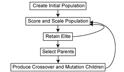
while programming also we use these steps to get the optimized solutions of the given function .

Syntax for the Genetic algorythm :-

ga(fun,nvars,Aineq,bineq,Aeq,beq,lb,ub,nonlcon,intcon)

fun -> Fitness function ( for eg , stalagmite function used in optimization )

nvars -> No. of variables

Aineq & bineq ->linear inequality constraints

Aeq & beq -> linear equality constraints

lb & ub -> lower and upper bound limits respectively.

nonlcon -> used for non linear constraints

intcon -> used to get the solution in integer

Code & Plot for all the three studies :-

CODE:-

clear all
close all
clc

% Now creating the search space for the function 

x = linspace(0,0.6,150);
y = linspace(0,0.6,150);
[X,Y] = meshgrid(x,y);

num_cases = 50; % Idea behind this is we will run the ga 50 times.
        
% Now drawing the surface plot for the stalagmite function 
%for this using teh For loop 
for i= 1:length(X)
    for j= 1:length(Y)
           input_vector(1)=X(i,j);
           input_vector(2)=Y(i,j);
           f(i,j)=stalagmite(input_vector); % we have given the value of function in the search space .
    end
end
% (-) negative sign is used to get the plot in the upside down direction to
% get the maxima .
surfc(X,Y,-f); %Creating the surface plot 
shading interp; % used to remove the grid lines on the plot.

% 1)Study for the statistical behaviour ( UNBOUNDED ) 
tic % using the tic & toc command for calculating the study time.
for i=1:num_cases
    % here we are calculating the optimised function 
    [inputs,fopt(i)]=ga(@stalagmite,2);
    xopt(i)=inputs(1);
    yopt(i)=inputs(2);
end
% this will display the respective time taken 
study1_time=toc

% Now plotting the graph for the Study ( 1 ) 
figure(1)
subplot(2,1,1);
surfc(X,Y,-f);
hold on
shading interp
plot3(xopt,yopt,-fopt,'marker','o','markersize',5,'markerfacecolor','r');
xlabel('x');
ylabel('y');
grid on 
subplot(2,1,1);
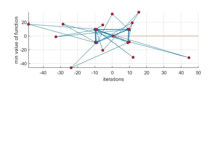
plot(-fopt);
xlabel('iterations');
ylabel('min value of function');

% 2)Study for the statistical behaviour ( BOUNDED )
tic
for j=i:num_cases
    [inputs,fopt(j)]=ga(@stalagmite,2,[],[],[],[],[0;0],[1;1]);
    xopt(j)=inputs(1);
    yopt(j)=inputs(2);
end
study2_time=toc

% Now plotting the graph for the Study ( 2 )
figure(2)
subplot(2,1,1);
hold on 
surfc(X,Y,-f)
shading interp
plot3(xopt,yopt,-fopt,'marker','o','markersize',5,'markerfacecolor','r');
xlabel('x');
ylabel('y');
grid on 
subplot(2,1,2);
plot(-fopt);
xlabel('iterations');
ylabel('min value of function');

% 3) Increasing the population size  ( Study 3 ) 
options= optimoptions('ga','PopulationSize',300);
tic
for k = 1:num_cases
    [inputs,fopt(k)]= ga(@stalagmite,2,[],[],[],[],[0;0],[1;1],[],[],options);
    xopt(k)=inputs(1);
    yopt(k)=inputs(2);
end
study3_time= toc

% Now plotting the graph for the Study ( 2 )
figure(3)
subplot(2,1,1)
hold on
surfc(X,Y,-f)
shading interp
plot3(xopt,yopt,-fopt,'marker','o','markersize',5,'markerfacecolor','r');
xlabel('x');
ylabel('y');
grid on 
subplot(2,1,2);
plot(-fopt);
xlabel('iterations');
ylabel('min value of function');

Code Expalaination :-

1. first three Commands are used to clear all the values, close all the figures and also clear the vlaues in teh command window .

2. After that creating the array x , y by using the linspace command which have 10 values in between 0 & 0.6 .

3. Now creating the 2 D array by using the above inputs and the meshgrid command

4. Assigning the number of cases so that we can run the ga 50 times

5.After this we have used the for loop to create the search space and give the values of the function . and also we have created the surface plot

6. Now for the statistical study 1 with unbounded condition , we have used the tic & toc command to study the time also we have used the for loop to make the ga run for 50 times and get the values of the function for every iteration .

7.after tghe for lopp in the study 1 we have plotted the plots by using the plot & plot3 ( this is used to plot the 3d graphs ) .

8. also the subplot command is used to view two different plots in same figure window , and also the x label and y label commands are ysed to specify the x and y axis .

9. in the ga we have also set upeer and the lower bound .

10. the same procedure is repeated for the dtudy 2

11. in the study 3 we have increased the population size and also optimoptions command is used to optimize the desired value.

12. similarly the plots have been plotted for the respective studies .

PLOTS :-

1st study

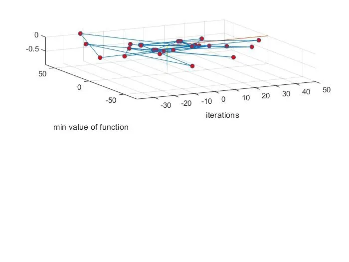
2nd study

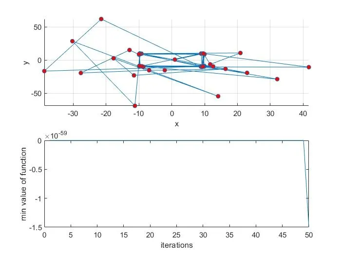
3rd study

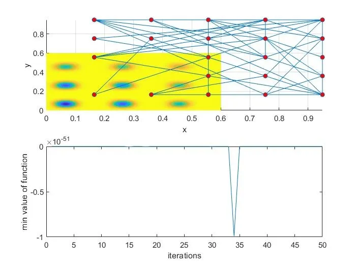
Error faced while coding : I faced the error that in the second and third study i am only getting the single plot in one figure and it was due to error in using the wrong value in subplot coammand " subplot() " .