Week 3 - Solving second order ODEs
Assuming the variables :
g = gravity in m/s2,
L = length of the pendulum in m,
m = mass of the ball in kg,
b=damping coefficient.
Programm for solving the above mentioned ODE ( for a simple pendulum ) :-
clear all
close all
clc

%Defining the variables
b=0.05;
g=9.81;
l=1;
m=1;

%Defining the initial conditions,angular displacement is zeroe and angular velocity is 5rad / second.

theta_0=[0;5];

%time span of 10 seconds
t_span=linspace(0,10,50);

% Solving the ODE ( for simple pendulum )
[t,result]=ode45(@(t,theta) ode_func(t,theta,b,g,l,m),t_span,theta_0)
Output :- we will get the values of angular displacement & angular velocity as the solutions for the sbove ODE .
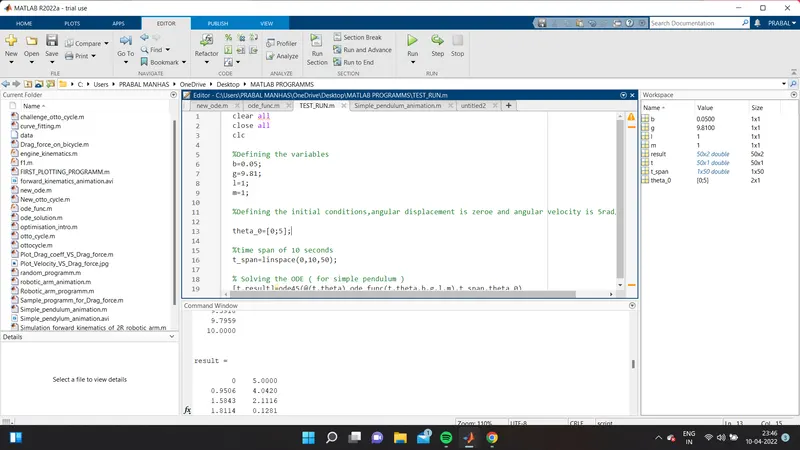
Explaination for the above programm :-
clear all (used to clear the variables from the current workspace )
close all (used to close all the figures )
clc (used to clear the command window)
%Defining the variables (%is used to add the comment as mentioned )
b=0.05;(value of b has been defined here )
g=9.81;(value of g has been defined here )
l=1;(value of l has been defined here )
m=1;(value of m has been defined here )
%Defining the initial conditions,angular displacement is zeroe and angular velocity is 5rad / second.
theta_0=[0;5];(defining the initial boundary conditions for angular displacement ,angular velocity )
%time span of 10 seconds
t_span=linspace(0,10,50);(value of t_span wil vary from 0 to 10 seconds , and will have 50 values in between )
% Solving the ODE ( for simple pendulum ) (% is used to add the comment )
[t,result]=ode45(@(t,theta) ode_func(t,theta,b,g,l,m),t_span,theta_0)
ode45 is an inbuilt solver for Ordinary differential Equations
@(t,theta ) defines the variables in ODE
ode_func is a function of t,theta,b,g,l,m that is called here
and then we have provided t_span as a integrating factor here
theta_0 is the initial boundary condition
note:- % is used to add the comment & ; is used to terminate the output in command window .
Programm for the ode_func ( that is used in above programm ) :-
function [dtheta_dt] = ode_func(t,theta,b,g,l,m)
theta1=theta(1);
theta2=theta(2);
dtheta1_dt=theta2;
dtheta2_dt=-(b/m)*theta2 -g/l*sin(theta1);
dtheta_dt=[dtheta1_dt; dtheta2_dt];
end
Function ( command is used to create the function )
[dtheta_dt] is the output of the ode_func.
dtheta1_dt = theta2 ( value of dtheta_dt has been defined )
dtheta2_dt = -(b/m)*theta2 -g/l*sin(theta1) ( value of dtheta2_dt has been defined here )
dtheta_dt=[dtheta1_dt; dtheta2_dt]; ( here dtheta_dt will the column vector having 2 balues in column )
End ( command is used to end the function )
Programm to simulate the pendulum Motion ( Animation ) :-
Assuming the values of
L=1 metre,
m=1 kg,
b=0.05.
g=9.81 m/s2
Time span varies between 0 to 20 seconds
angular displacement=0,angular velocity=3 rad/sec at time t=0 [ initial boundary condition ]
close all
clear all
clc

% Defining the inputs
l=1;
m=1;
b=0.05;
g=9.81;

% As per given initial Boundary condition
theta_0=[0;3];
% the time span needs to be 20 seconds
t_span=linspace(0,20,100);

% solving 2nd ode ,for pendulum
[t,result]= ode45(@(t,theta) ode_func(t,theta,b,g,l,m),t_span,theta_0);

% creating plots for tracing angular velocity and angular displacement .
subplot(2,1,1);
plot(t,result(:,l),'LineWidth',3);
xlabel('Time in seconds');
ylabel('Angular displacement');
subplot(2,1,2);
hold on;
plot(t,result(:,2),'LineWidth',3);
xlabel('Time in seconds');
ylabel('Angular velocity');
grid on;

% animation process
X0=0;
Y0=0;
ct=1;

for i=1:length(t)

    X1=l*sin(result(i,1));
    Y1=-l*cos(result(i,1));

    figure(2)
    plot([-1 1],[0 0],'linewidth',6,'color','r');
    axis([-2 2 -2 2]);
    line([X0,X1],[Y0,Y1],'linewidth',2,'color','b');
    hold on
     plot(X0,Y0,'O','markersize',3,'markerfacecolor','y');
    plot(X1,Y1,'O','markersize',20,'markerfacecolor','g');
    title('Graph showing animation of simple pendulum');
    legend('support rod','length of string','fixed point','bob of pendulum');
    grid on;

    hold off ;
    pause(0.1);
    M(ct)=getframe(gcf);
    ct=ct +1;
end
 movie(M)
videofile = VideoWriter('Simple_pendylum_animation.avi','uncompressed AVI');
open(videofile)
writeVideo(videofile,M)
close(videofile)
Explaination of the code :-
close all (used to close all the figures )
clear all (used to close all the figures )
clc (used to clear the command window)
% Defining the inputs
l=1;( where l is the length of the string and it is defined here )
m=1; (where m is the mass and it is defined here )
b=0.05; (where b is the damping coeff.and it is defined here )
g=9.81; (this is acc. due to gravity and it has also been defined here )
% As per given initial Boundary condition
theta_0=[0;3];(theta_0 will be array of 2 rows & 1 column , denotes the value of angular displacement & angular velocity respectively )
% the time span needs to be 20 seconds
t_span=linspace(0,20,100);(using the linspace command to create an array starting from 0 and ending to 20 having 100 values in between )
% solving 2nd ode ,for pendulum
[t,result]= ode45(@(t,theta) ode_func(t,theta,b,g,l,m),t_span,theta_0);
ode45 is an inbuilt solver for Ordinary differential Equations
@(t,theta ) defines the variables in ODE
ode_func is a function of t,theta,b,g,l,m that is called here
and then we have provided t_span as a integrating factor here
theta_0 is the initial boundary condition
% creating plots for tracing angular velocity and angular displacement .
subplot(2,1,1); ( used to create the subplots in 2 by 1 grid in 1 axis )
plot(t,result(:,l),'LineWidth',3); (used to create the plot between t,1st column of result which shows the values of angular displacement )
xlabel('Time in seconds'); ( writing the x axis label )
ylabel('Angular displacement'); (writing the y axis label )
subplot(2,1,2);( used to create the subplots in 2 by 1 grid in 2 axis )
hold on; ( used to hold the current figure )
plot(t,result(:,2),'LineWidth',3);(used to create the plot between t,2nd column of result which shows the values of angular velocity )
xlabel('Time in seconds');( writing the x axis label )
ylabel('Angular velocity');(writing the y axis label )
grid on;( used to on the grids )
% animation process
X0=0;( defining the x0 to be 0)
Y0=0;( defining the y0 to be 0)
ct=1; ( loop counter)
for i=1:length(t) ( starting the loop , which means for the value from 1 to the values in t , i will be assigned )
X1=l*sin(result(i,1));( defining the coordinates & position of pendulum in x axis )
Y1=-l*cos(result(i,1));( defining the coordinates & position of pendulum in y axis )
figure(2) ( used to create a different figure )
plot([-1 1],[0 0],'linewidth',6,'color','r'); ( used to create the plot having values -1 to 1 in x axis & 0 in y axis , linwidth command is used to incresed the width of the line )
axis([-2 2 -2 2]);( setting the axis limits )
line([X0,X1],[Y0,Y1],'linewidth',2,'color','b');( used to create the line between two end points { (x0,y0) & (x1,y1) }
hold on ( used to hold the current figure )
plot(X0,Y0,'O','markersize',3,'markerfacecolor','y');(plotting the fixed point , and highlighting it with marker whose size is 3 and colour is yellow )
plot(X1,Y1,'O','markersize',20,'markerfacecolor','g');(plotting the cordinates x1,y1 , and highlighting it with marker whose size is 20 and colour is green )
title('Graph showing animation of simple pendulum');(used for giving the title to the graph )
legend('support rod','length of string','fixed point','bob of pendulum');(used to highlight the lines used in the graph to specify support rod ,length of string , fixed point , bob of pendulum )
grid on; (used to turn on the grids )
hold off ;(used to turn off the hold command )
pause(0.1); (pausing the code by factor 0.1 )
M(ct)=getframe(gcf);( creating and sacing the frames in M(ct))
ct=ct +1;(incrementing the counter by 1, when the lopp repeats )
end (used to end up the for loop )
movie(M)(creating the movie of M )
videofile = VideoWriter('Simple_pendylum_animation.avi','uncompressed AVI'); (saving the videofile, with name Simple_pendylum_animation.avi )
open(videofile)( giving command to open the file )
writeVideo(videofile,M) ( write in the video file )
close(videofile) ( closing the video file )
Output of the above code : -
1.Plots will be plotted between ( time ,angular displacement) & ( time , angular velocity )
2. Animation will be there for a simple pendulum .
1.RESPECTIVE PLOTS
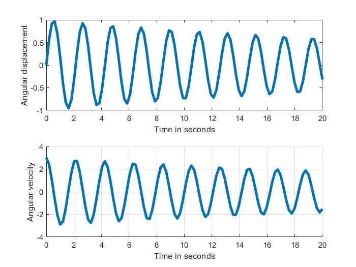
2.ANIMATION VIDEO LINK :- https://youtu.be/gedaoKyUTfA
Errors faced while Programming :-
1. 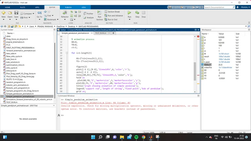
this error arises due wrong syntax use , i forgot to put the single inverted comma both side while linewidth .
'linewidth ( wrong usage )
'linewidth' ( correct usage )
2.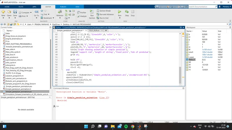
This error arised when I used Movie instead of movie , that fuction is not known to matlab , thats why throwing the error unrecognised fuction or variable .