Project 2 - Rankine cycle Simulator
RANKINE CYCLE SIMULATOR :-
CODE :-
clear all
close all
clc

% Displaying the processes involved
disp('Rankine Cycle Simulator');
disp('1-2 Isentropic expansion int the turbine');
disp('2-3 Heat removal process in the condenser at constant pressure');
disp('3-4 is the isentropic compression in the pump');
disp('4-1 Heat addition Process in the boiler at constant pressure');

% Now getting the data for input,WE have already given the values of these inputs in the challenge
p1=44; % inlet pressure of the turbine in bars
t1=538; % Inlet temprature of the Turbine in degree celsius
p2=5.83; % inlet pressure for condensor in bars

% Now extracting the data and defining the variables
% For state 1
h1=XSteam('h_pt',p1,t1); % where h is for enthalpy
s1=XSteam('s_pt',p1,t1);% where s is for entropy

% Now extracting the data and defining the variables
% For state 2
s2=s1; % due to isentropic expansion

sf2=XSteam('sL_p',p2);% Entropy for saturated liquid
sg2=XSteam('sV_p',p2);% Entropy for saturated vapour
x2=(s2-sf2)/(sg2-sf2);
hf2=XSteam('hL_p',p2);% Enthalpy for saturated vapour
hg2=XSteam('hV_p',p2);% Enthalpy for saturated vapour
h2=hf2 + (x2*(hg2-hf2));

% Now extracting the data and defining the variables
% For state 3
p3=p2; % due to heat rejection in condenser at constant pressure
s3=XSteam('sL_p',p3);
h3=XSteam('hL_p',p3);

% Now extracting the data and defining the variables
% For state 4
s4=s3; % due to isentropic compression
p4=p1;% due to heat addition at constant pressure

% Now calculating the work done (wd) by the turbine
wd=h1-h2;

% Now calculating the work done (wp) to run pump
v3=XSteam('vL_p',p3);
wp=v3*(p4-p3)*100;
h4=h3+wp;

% Now calculating the net workdone ( w_net)
w_net=wd-wp;

% calculating the heat input ( q_input ) to the system
q_input=h1-h4;

% calculating the heat input ( q_output ) to the system
q_output=h2-h3;

% Now calculating the thermal efficiency
Thermal_eff= (w_net/q_input)*100;

% Now calculating the specific steam consumption (sc_specific)
%formula used is :sc_specific= mass flow rate /power
sc_specific=(3600/w_net);

% Hence we are only left with the values of temprature at different states
% so Now moving forward to calculate the temprature values respectively
t3=XSteam('Tsat_p',p3);
t2=t3;
cp4=XSteam('cp_ps',p4,s4);% specific heat at constant pressure
cv4=XSteam('cv_ps',p4,s4);% specific heat at constant volume
k=cp4/cv4; % Heat capacity ratio
t4=t3/(p3/p4)^((k-1/k));

% Now calculating the temprature , entropy, enthalpy at the vapour and the
% liquid line for the plotting purpose
t6=XSteam('Tsat_p',p1);
t5=t6;
s5=XSteam('sL_p',p1);
s6=XSteam('sV_p',p1);
h5=XSteam('hl_p',p1);
h6=XSteam('hV_p',p1);

%% Now plotting the saturation curve
t=linspace(1,380,1000);
for i=1:length(t)
    sf(i)=XSteam('sL_t',t(i));
    sg(i)=XSteam('sV_t',t(i));
    hf(i)=XSteam('hL_t',t(i));
    hg(i)=XSteam('hV_t',t(i));
end

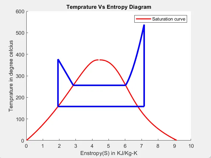
%% Now plotting the t-s Diagram
figure(1)
hold on
plot(sf,t,'r','linewidth',2);
plot(sg,t,'r','linewidth',2);
plot([s1 s2],[t1 t2],'b','LineWidth',3);
plot([s2 s3],[t2 t3],'b','LineWidth',3);
plot([s3 s4],[t3 t4],'b','LineWidth',3);
plot([s4 s5],[t4 t5],'b','LineWidth',3);
plot([s5 s6],[t5 t6],'b','LineWidth',3);
sc1=linspace(s6,s1,1000);
for j=1:length(sc1)
    tc1 (j)=XSteam('T_ps',p1,sc1(j));
end
plot(sc1,tc1,'b','linewidth',3);
title('Temprature Vs Entropy Diagram');
xlabel('Enstropy(S) in KJ/Kg-K');
ylabel('Temprature in degree celcius');
legend('Saturation curve');

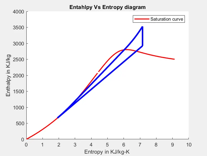
%% Now plotting the H-S Diagram
figure(2)
hold on
plot(sf,hf,'r','lineWidth',2);
plot(sg,hg,'r','linewidth',2);
plot([s1 s2],[h1 h2],'b','linewidth',3);
plot([s2 s3],[h2 h3],'b','linewidth',3);
plot([s3 s4],[h3 h4],'b','linewidth',3);
hc=linspace(h4,h5,1000);
for k=1:length(hc)
    sch(k)=XSteam('s_ph',p1,hc(k));
end
plot(sch,hc,'b','LineWidth',3);
plot([s5 s6],[h5 h6],'b','LineWidth',3);
for m=1:length(sc1)
    hc1(m)=XSteam('h_ps',p1,sc1(m));
end
plot(sc1,hc1,'b','linewidth',3);
title('Entahlpy Vs Entropy diagram');
xlabel('Entropy in KJ/kg-K ');
ylabel('Enthalpy in KJ/kg');
legend('Saturation curve');

% Displaying the results as per input
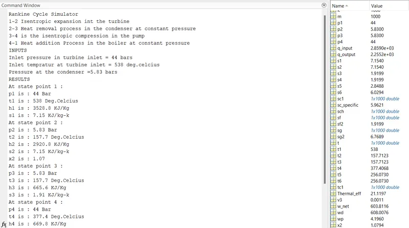
disp('INPUTS')
disp('Inlet pressure in turbine inlet = 44 bars')
disp('Inlet tempratur at turbine inlet = 538 deg.celcius')
disp('Pressure at the condenser =5.83 bars')
disp('RESULTS')

%At state 1
disp('At state point 1 :')
disp('p1 is : 44 Bar')
disp('t1 is : 538 Deg.Celcius')
disp('h1 is : 3528.8 KJ/Kg') %% Calculated the value mannually by converting 3.5288e+03
disp('s1 is : 7.15 KJ/kg-k')

%At state 2
disp('At state point 2 :')
disp('p2 is : 5.83 Bar')
disp('t2 is : 157.7 Deg.Celcius')
disp('h2 is : 2920.8 KJ/Kg')%% Calculated the value mannually by converting 2.9208e+03
disp('s2 is : 7.15 KJ/kg-k')
disp('x2 is : 1.07')

%At state 3
disp('At state point 3 :')
disp('p3 is : 5.83 Bar')
disp('t3 is : 157.7 Deg.Celcius')
disp('h3 is : 665.6 KJ/Kg')
disp('s3 is : 1.91 KJ/kg-k')

%At state 4
disp('At state point 4 :')
disp('p4 is : 44 Bar')
disp('t4 is : 377.4 Deg.Celcius')
disp('h4 is : 669.8 KJ/Kg')
disp('s4 is : 1.91 KJ/kg-k')


disp('wd is :608 kj/kg') % here wd is used in place of wt
disp('wp is :4.19 kj/kg')
disp('w_net is :603.8 kj/kg')
disp('Thermal_eff is  :21.11 Percent')% here Themal_eff isused in place of Nthermal
disp('sc_specific is :5.96')% here sc_specific is used in place of SSC.
EXPLAINATION OF CODE & LOGIC :-

The Rankine cycle is an idealized thermodynamic cycle describing the process by which certain heat engines, such as steam turbines or reciprocating steam engines, allow mechanical work to be extracted from a fluid as it moves between a heat source and heat sink. The Rankine cycle is named after William John Macquorn Rankine, a Scottish polymath professor at Glasgow University.
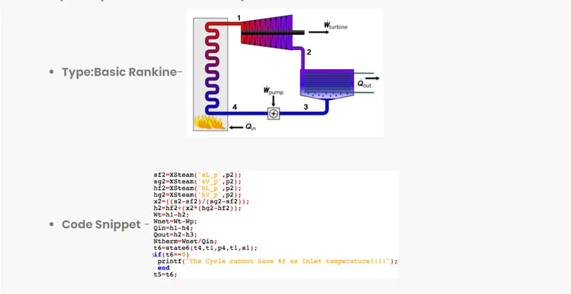
Heat energy is supplied to the system via a boiler where the working fluid (typically water) is converted to a high pressure gaseous state (steam) in order to turn a turbine. After passing over the turbine the fluid is allowed to condense back into a liquid state as waste heat energy is rejected before being returned to boiler, completing the cycle. Friction losses throughout the system are often neglected for the purpose of simplifying calculations as such losses are usually much less significant than thermodynamic losses, especially in larger systems
Working Process can be explained with the below Screen shot:-
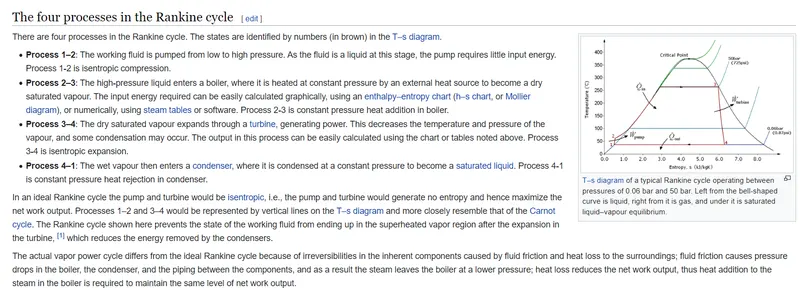
Also used this helpfull info provided in the challenge and also very thankfull for providing this info :
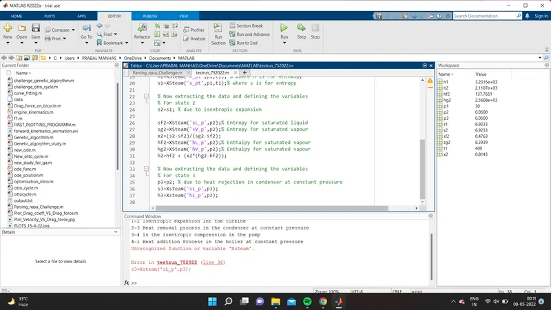
Error faced :- the error i faced was , i am using the wrong keyword ie Xsteam, instead of XSteam , which has caused a lot of problem .
References :-
https://en.wikipedia.org/wiki/Rankine_cycle