Week 4.1 - Genetic Algorithm

Aim- To write a code in Matlab to optimise the Stalagmite function and find the Global maxima of the function.

Objective -

• To optimise the stalagmite function and find the global maxima of the function .
• Explain the Concept of Genetic Algorithm & Explain the syntax for ga in Matlab.
• Plot the Graphs for F Maximum vs no. Of Iterations.

Theory-

Genetic Algorithm-

The Genetic algorithm is a method for both constrained and unconstrained optimization problems that is based on natural selection , The process that drives biological evolution. The Genetic algorithm repeatedly modifies a population of individual Solutions. the genetic algorithm selects individuals from the current population to be parents and uses them to produce the children for the next generation. over successive generations ,the population 'evolves' towards an optimal solution .

genetic algorithm can apply to solve a variety of optimization problems that are not well suited for standard optimization algorithms, including problems in which the objective function is discontinuous, nondifferentiable, stochastic or highly nonlinear .

Introduction to Optimization - Optimization is the process of making something better. In any process, we have a set of inputs and a set of outputs.

Optimization refers to finding the values of inputs in such a way that we get the best output values. the Definition of best varies from problem to problemproblem, but in mathematical terms , it refers to maximizing or minimizing one or more objective functions by varying the input parameters.

Advantages of Genetic Algorithm -

• Does not require any derivative information.
• It is faster and more efficient as compared to the traditional method.
• Has very good Parallel capabilities.
• Provides a list of good solutions and not just a single solution.
• Always gets an answer to the problem, which gets better over the time.

Limitations of Genetic Algorithm -

• GA's are not suited for all problems, especially problems which are simple and for which derivative information is avilable.
• Fitness value is calculated repeatedly which might be computationally expensive for some problems.
• Being stochastic there are no guarantees on the optimality or the quality of the solution.
• if not implemented properly, the GA may not converge to the optimal solution.

Input function -

`F(x, y) = f1, x*f2, x*f1, y*f2, y`

Where,

`f1, x`= `[Sin(5.1pix+0.5) ]^6`

`f1, y`=`[Sin(5.1piy+0.5) ]^6`

`f2, x` =`exp [((-4ln(2) (x-0.667) ^2) /(0.64)) ]`

`f2, y` = `exp[((-4ln(2) (y-0.667) ^2) /0.64) ]`

stalagmite function Code -

function[f]=stalagmite(input_vector)

x=input_vector(1);
y=input_vector(2);

f1.x=(sin(5.1*pi*x+0.5)).^6;

f1.y=(sin(5.1*pi*y+0.5)).^6;

f2.x= exp(-4*log(2)*((x-0.0667).^2)/0.64);
f2.y = exp(-4*log(2)*((y-0.0667).^2)/0.64);

f= -(f1.x*f1.y*f2.x*f2.y)
end

basic code-

clear all
close all
clc

% Defining our search space

x=linspace(0,0.6,150);
y=linspace(0,0.6,150);

% creating a 2Dimensional mesh
[xx yy]= meshgrid(x,y);

%Evaluating the stalagmite function

for i=1:length(xx);
    for j=1:length(yy);
        input_vector(1) = xx(i,j);
        input_vector(2) = yy(i,j);
        f(i,j)= stalagmite(input_vector);
    end
end

surfc(xx,yy,f)
shading interp
xlabel('x value');
ylabel('y value');
[inputs,fval]= ga(@stalagmite,2)

main code-

clear all
close all
clc

x=linspace(0,0.6,150);
y=linspace(0,0.6,150);

num_cases=50;
% Creating a 2Dimensional mesh 
[xx yy]= meshgrid(x,y);

%Evaluating the stalagmite function
for i=1:length(xx);
    for j=1:length(yy);
        input_vector(1) = xx(i,j);
        input_vector(2) = yy(i,j);
        f(i,j)= stalagmite(input_vector);
    end
end


tic
%study 1-statistical behavior

for i=1:num_cases
    [inputs, fopt(i)]= ga(@stalagmite,2);
    xopt(i)=inputs(1);
    yopt(i)=inputs(2);

end
study1_time=toc
figure(1);
subplot(2,1,1);
hold on
surfc(x,y,f)
shading interp
plot3(xopt,yopt,-fopt,'marker','o','MarkerSize',5,'MarkerFaceColor','r');

title('Unbounded Inputs')
subplot(2,1,2)
plot(-fopt)
xlabel('Iterations')
ylabel('Function minimum')

tic
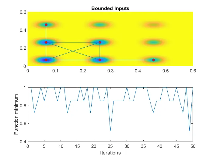
% study 2-statistical behavior with upper and lower bounds
for i=1:num_cases
    [inputs,fopt(i)]=ga(@stalagmite,2,[],[],[],[],[0;0],[1;1]);
    xopt(i)=inputs(1);
    yopt(i)=inputs(2);
end

study2_time=toc

figure(2)
subplot(2,1,1)
hold on
surfc(x,y,f)
shading interp
plot3(xopt,yopt,-fopt,'Marker','o','MarkerSize',5,'MarkerFaceColor','r')
title('Bounded Inputs')
subplot(2,1,2)
plot(-fopt)
xlabel('Iterations')
ylabel('Function minimum')

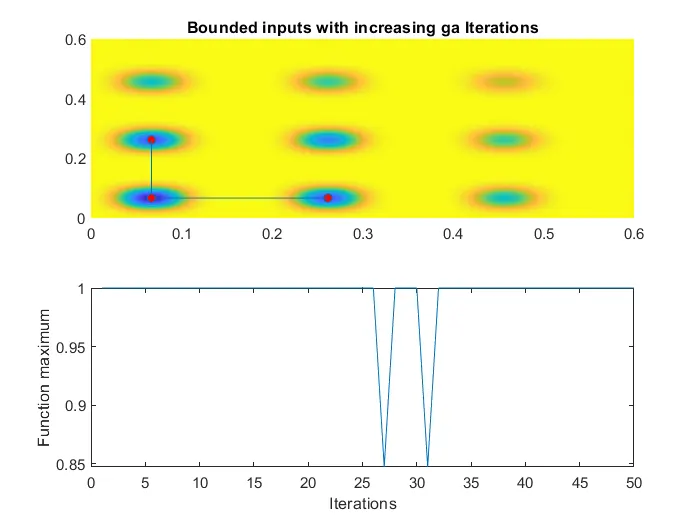
% study 3 increasing ga iterations
options=optimoptions('ga')
options=optimoptions(options,'Populationsize',170);

tic
for i=1:num_cases
    [inputs,fopt(i)]=ga(@stalagmite,2,[],[],[],[],[0;0],[1;1],[],[],options);
    xopt(i)=inputs(1);
    yopt(i)=inputs(2);
end

study3_time=toc
figure(3)
subplot(2,1,1)
hold on
surfc(x,y,f)
shading interp
plot3(xopt,yopt,-fopt,'marker','o','markersize',5,'MarkerFaceColor','r');
title('Bounded inputs with increasing ga Iterations')
subplot(2,1,2)
plot(-fopt)
xlabel('Iterations')
ylabel('Function maximum')

Output-

basic -

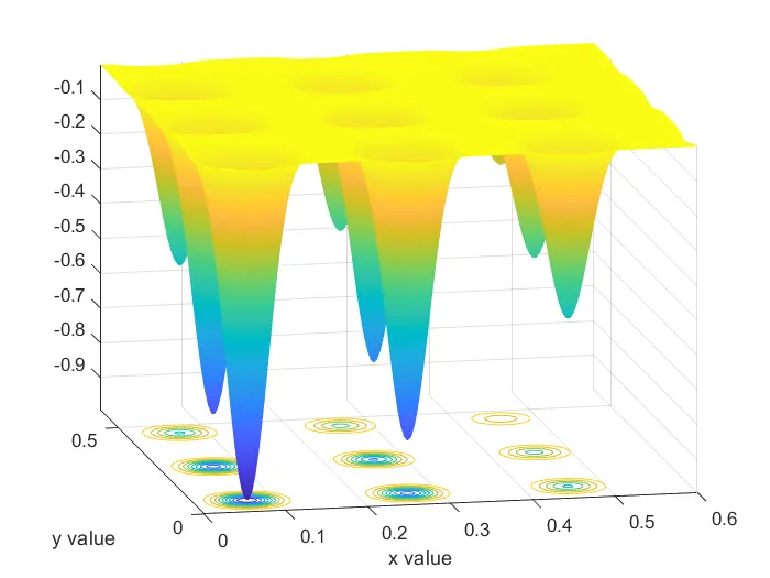
unbounded Statistical behaviour plot -

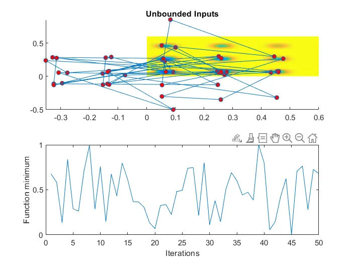
Bounded Statistical Behaviour Plot-

Modified Population size plot-

Optimization terminated: average change in the fitness value less than options.FunctionTolerance.

study3_time =

87.0246