Project 2 - Rankine cycle Simulator

Aim-

• To simulate a Rankine cycle using Matlab using Xsteam data
• calculate all the state points of the cycle
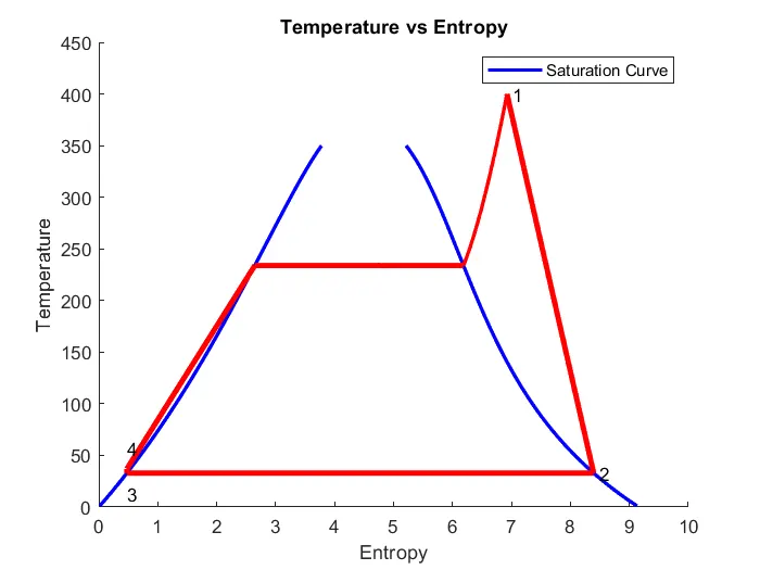
• plot T vs S and H vs S plots for rankine cycle

Theory-

Rankine cycle is a idealized thermodynamic cycle in which a fluid is used to produce heat in boiler , converting water into extreme heat vapour to start a turbine . turbine used that heat to produce mixture of less heat and vapour than it goes through condenser in which subcooled area the heat is converted into liquid state and it is work done to flow the water to pump. it is closed cycle.

rankine cycle is derived out of carnot cycle.

it has four processes-

(1-2)- Isentropic Expansion

(2-3)- Constant pressure heat rejection

(3-4)- Isentropic Compression

(4-1)- constant pressure heat addition

Program-

clear all
close all
clc

% Process information

fprintf('1-2 Isentropic Expansion\n')
fprintf('2-3 Constant Pressure Heat Rejection\n')
fprintf('3-4 Isentropic Compression\n')
fprintf('4-1 Constant Pressure Heat Addition\n')

% Input description
p1= (' Enter the Pressure at the turbine inlet(in bar)=');
T1= (' Enter the Temperature at the turbine inlet(in degree celcius)=');
p2= (' Enter the Pressure at the outlet of condenser(in bar)=');

% calculate each state points
p1=30;
T1=400;
p2=0.05;


%state point 1
h1= XSteam('h_pT',p1,T1);
s1=XSteam('s_pT',p1,T1);

%state point 2
s2=s1
sf2= XSteam('sL_p',p2);
sg2=XSteam('sV_p',p2);
hf2= XSteam('hL_p',p2);
hg2=XSteam ('hV_p',p2);     %x2=(s2-sf2)/(sg2-sf2);

s2=sg2;
h2=hg2;        %hf2+(x2*(hg2-hf2));

%state point 3

p3=p2;
s3=XSteam('sL_p',p3);
h3=XSteam('hL_p',p3);
v3=XSteam('vL_p',p3);

%state point 4

s4=s3;
p4=p1;


%calculating temperatures

T3=XSteam('Tsat_p',p3);
T2=T3;
cp4=XSteam('cp_ps',p4,s4);
cv4=XSteam('cv_ps',p4,s4);
gamma=cp4/cv4;
r=(gamma-1)/gamma;
T4=T3*(p4/p3)^r;


% work done by turbine
wt=h1-h2;

%workdone to flow water to pump
wp= v3*(p4-p3)*100;

h4=wp+h3;

% Net work done 
wnet=wt-wp;

% Heat input to the system

Qin=h1-h4;

% Heat rejection 

Qout=h2-h3;

% Thermal Efficiency
efficiency=(wnet/Qin)*100;

%specific steam consumption

%SSC= mass flow rate / power

SSC= (3600/wnet);

%state point 5 and 6


T6=XSteam('Tsat_p',p1);
T5=T6;
s5=XSteam('sL_p',p1);
s6=XSteam('sV_p',p1);
h5=XSteam('hL_p',p1);
h6=XSteam('hV_p',p1);

% plotting the saturation curve
T=linspace(1,350,1000);
for i=1:length(T)

    sf(i)=XSteam('sL_T',T(i));
    sg(i)=XSteam('sV_T',T(i));
    hf(i)=XSteam('hL_T',T(i));
    hg(i)=XSteam('hV_T',T(i));
end

% plotting T-S diagram

figure(1)
hold on
plot(sf,T,'b','linewidth',2)
plot(sg,T,'b','linewidth',2)
plot([s1 s2],[T1 T2],'r','linewidth',3)
plot([s2 s3],[T2 T3],'r','linewidth',3)
plot([s3 s4],[T3 T4],'r','linewidth',3)
plot([s4 s5],[T4 T5],'r','linewidth',3)
plot([s5 s6],[T5 T6],'r','linewidth',3)

sp1=linspace(s6,s1,1000);
for j= 1:length(sp1)
    Tp1(j)=XSteam('T_ps',p1,sp1(j));
end

plot(sp1,Tp1,'r','LineWidth',2)
text(s1+0.1,T1,'1')
text(s2+0.1,T2,'2')
text(s3,T3-20,'3')
text(s4,T4+20,'4')

title('Temperature vs Entropy')
xlabel('Entropy')
ylabel('Temperature')
legend('Saturation Curve')

results-