Week 3 - Solving second order ODEs

Aim - To solve the second Order Differential Equation(ODE) using the matlab which represents the equation of motion of a simple pendulum with damping.

Governing Equations- The second order differential equation is defined as-

`(d^2theta)/dt^2 +(b/m)(d theta)/dt +g/lsintheta`=0

where,

b= damping co-efficient

m= mass(kg)

g= Gravity (`m/sec^2`)

l= Length(meter)

the above equation after break into two 1 order equations

let `theta=theta1`

`(d theta)/dt`= `(d theta1)/dt`=`theta2` ............(1)

(`(d^2theta)/dt^2`)=(`(d^2theta1)/dt^2`)= `d/dt``(d theta1)/dt`=`d/dt``(theta2)` ............(2)

therefore our 2nd order differential equation-

`(d^2theta)/dt^2 +(b/m)(d theta)/dt +g/lsintheta`=0

substituting the above two equations into second order differential equation-

`(d^2theta1)/dt^2` + `b/m((d theta1)/dt)`+`(g/l)sintheta`=0

`((d theta2)/dt)+((b/m)theta2)+ (g/l)sintheta1`=0

therefore,

`(d theta1)/dt=theta2`

`((d theta2)/dt)= -b/m theta2 -(g/l)sin theta1`

now we have theta1 & theta2

Objectives-

• to write a program that solves the ODE of motion of simple pendulum with damping
• Plot the graph of the angular displacement & angular velocity w.r.t. to time
• Create an animation to simulate the motion of pendulum

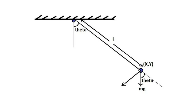
a simple pendulum consists of a bob of mass m , string of length l, the gravitational force is g .

Body of the content-

Programing Language used in this program is 'Matlab'

now the code is -

clear all
close all
clc

b=0.05;
g=9.81;
l=1;
m=1;

% Initial Condition
theta_0=[0;3];

% Time points
t_span= linspace(0,20,300);

% Solve ODE
[t,results]= ode45(@(t,theta) ode_func(t,theta,b,g,l,m),t_span,theta_0);
plot(t,results(:,1))
hold on
plot(t,results(:,2))
xlabel('time')
ylabel('plot')
legend('angular displacement','angular velocity')

% for loop for oscillation of pendulum
ct=1;

for i=1:length(results(:,1))
    % coordinates for fixed axis
    x0=0;
    y0=0;

    % coordinates
    x1=l*sin(results(i,1));
    y1= -l*cos(results(i,1));

% plotting the animation
figure(2)
    plot([-1 1],[0 0],'linewidth',3)
    hold on

    plot([x0 x1],[y0 y1],'linewidth',3,'color','b')

   hold on
    plot(x1,y1,'marker','o','Markersize',30,'markerfacecolor','r')
     axis([-2 2 -2 1]);
   
    pause(0.03);
    hold off
    title({'simple harmonic motion of a pendulum'},'color','g')
  
  
    M(ct)=getframe(gcf);
    ct=ct+1;

end

% converting the animation into movie
movie(M)
Videofile= VideoWriter('Pendulum_motion.avi','Uncompressed AVI');
open(Videofile)
writeVideo(Videofile,M)
close(Videofile)

The Function code used in this Program-

function[dtheta_dt]= ode_func(t,theta,b,g,l,m)

theta1=theta(1)
theta2=theta(2)
dtheta1_dt = theta2;
dtheta2_dt= -(b/m)*theta2-(g/l)*sin(theta1);

dtheta_dt =[dtheta1_dt;dtheta2_dt];
end

Errors, i faced during programing

this error was showing because i run the program without introduce the function code.

Solution-

Introduce the function code than run the program.

Results-

The plot of Angular Displacement and Angular Velocity has obtained and it is showing oscillations of simple pendulum.

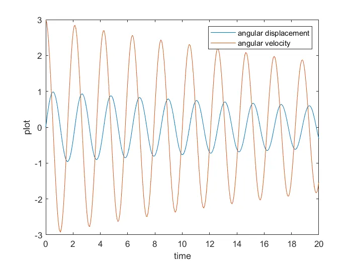
The animated video of the simple pendulum is mentioned below in this youtube link-

https://www.youtube.com/watch?v=p2HR7SLvq5k

Conclusion-

Using Matlab we have solved the second order differential equation and we have obtained a Graph which is showing oscillations of simple pendulum and showing oscillations in angular displacement and angular velocity.

we have created a animated movie of the motions of simple pendulum.