Objectives :-
To write a code to optimize the stagalmite function and maximize the global maxima.
Requirements:-
- Explanation od genetic algorithm and syntax in matlab
- make sure the program gives thw same output for any no of iterations
- plot all 3 graphs , f-maxima Vs no. of ierations with the title, legend,axes 7 labels.
Algorithm:-
is based on the evolution theory, this technique is used for solving noth constrained and unconstrained optimization problems , based on natural selection, the process that runs the biological evolution
- selection rule
- cross over rule
- mutation rule
find the local manima which is found to varry each time we run the programe the consistancy of this can be improved by , increasing the population size, asigning the boundedless, changing the mutation and crossover rate.
Syntax :- var_x = ga(@functions,nvars,A,b,Aeq,beq,lb,ub,nonicon,lntcon,options)
@function : The Function to be alaysed to find the minima.
nvars: This represnts the number of the variables to be evaluated.
A,b : This shows the linear inequality constraints.
Aeq,beq : This represnts the linear equalities.
lb,ub : Represents the lower and upper bound values in which the function is to evaluated.
nonicon : This shows the non linear constraints.
lntcon : This reprents the integer constraints.
options: thease are the options necessary for optimising the algorithm such as population size , cross over function.
Stagalmite Function :-
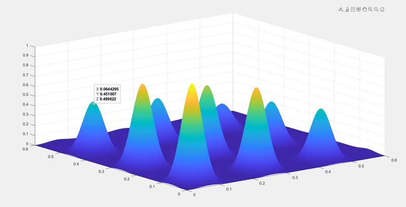
- A Stagalmite is an upward-growing mound of mineral deposits that have precipitated from water dripping onto the floor of a cave most stagalmite have rounded or flattened tips.
- A stagalmite function refers to the function with which are generating values over a stagalmite kind of surface for finding out the local and global maxima and minima of that particularly given function.
- in Matlab we use a method called optimization , it is programming that does a selection of the best element with regard to same criteria from the some set of population.
Code :-
clear all
close all
clc
% Writing optimization program
% range of x
x=linspace(0,0.6,150);
% range of y
y=linspace(0,0.6,150);
[xx, yy]=meshgrid(x,y);
% Evaluating Stalagmite Function.
for i=1:length(xx)
for j=1:length(yy)
input_vector(1)=xx(i,j);
input_vector(2)=yy(i,j);
f(i,j)=stalagmite_function(input_vector);
end
end
surf(xx,yy,-f);
shading interp;
[x,fval] = ga(@stalagmite_function,2);
% Optimization Program
x=linspace(0,0.6,150);
y=linspace(0,0.6,150);
[xx,yy] = meshgrid(x,y);
% Evaluating Stalagmite Function
for i=1:length(xx)
for j=1:length(yy)
input_vector(1)=xx(i,j);
input_vector(2)=yy(i,j);
f(i,j)=stalagmite_function(input_vector);
end
end
surf(xx,yy,-f);
hold on
shading interp;
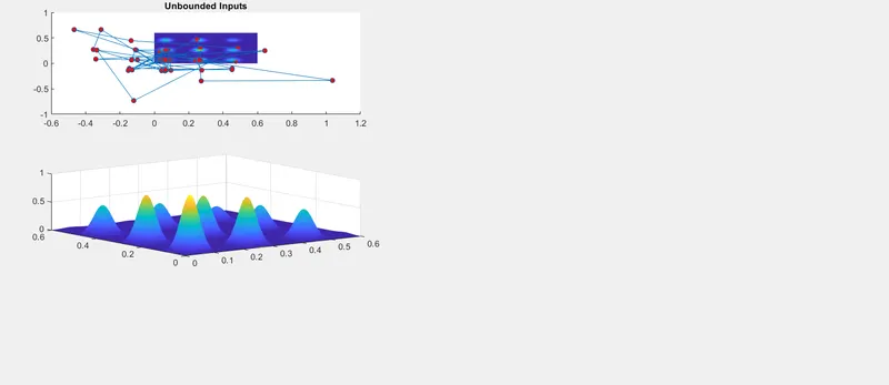
% Unbounded
tic
num_cases = 50;
for i=1:num_cases
[results,fopt(i)] = ga(@stalagmite_function,2);
xopt(i)=results(1);
yopt(i)=results(2);
end
study_time1 = toc
figure(2);
subplot(2,1,1)
hold on
surf(xx,yy,-f);
shading interp;
plot3(xopt,yopt,-fopt,'marker','o','markersize',5,'markerfacecolor','r');
title('Unbounded Inputs');
subplot(2,1,2);
plot(-fopt);
xlabel('Iterations');
ylabel('Function Maximum Value');
% Bounded Solutions
x=linspace(0,0.6,150);
y=linspace(0,0.6,150);
[xx,yy] = meshgrid(x,y);
% Evaluating Stalagmite Function
for i=1:length(xx)
for j=1:length(yy)
input_vector(1)=xx(i,j);
input_vector(2)=yy(i,j);
f(i,j)=stalagmite_function(input_vector);
end
end
surf(xx,yy,-f);
hold on
shading interp;
tic
num_cases = 50;
for i=1:num_cases
[results,fopt(i)] = ga(@stalagmite_function,2,[],[],[],[],[0,0],[0.6,0.6]);
xopt(i)=results(1);
yopt(i)=results(2);
end
Study_time1 = toc
figure(2);
subplot(2,1,1)
hold on
surf(xx,yy,-f);
shading interp;
plot3(xopt,yopt,-fopt,'marker','o','markersize',5,'markerfacecolor','r');
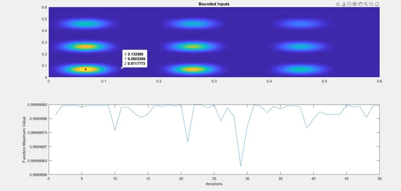
title('Bounded Inputs');
subplot(2,1,2);
plot(-fopt);
xlabel('Iterations');
ylabel('Function Maximum Value');
% Optimization Program
x=linspace(0,0.6,150);
y=linspace(0,0.6,150);
[xx,yy] = meshgrid(x,y);
% Evaluating Stalagmite Function
for i=1:length(xx)
for j=1:length(yy)
input_vector(1)=xx(i,j);
input_vector(2)=yy(i,j);
f(i,j)=stalagmite_function(input_vector);
end
end
surf(xx,yy,-f);
hold on
shading interp;
% Optimization
options = optimoptions('ga');
options = optimoptions(options,'PopulationSize',200);
tic
num_cases = 50;
for i=1:num_cases
[results,fopt(i)] = ga(@stalagmite_function,2,[],[],[],[],[0,0],[0.6,0.6],[],[],options);
xopt(i)=results(1);
yopt(i)=results(2);
end
Study_time1 = toc
figure(3);
subplot(2,1,1)
hold on
surf(xx,yy,-f);
shading interp;
plot3(xopt,yopt,-fopt,'marker','o','markersize',5,'markerfacecolor','r');
title('Bounded Inputs');
subplot(2,1,2);
plot(-fopt);
xlabel('Iterations');
ylabel('Function Maximum Value');
%stalgmite function code
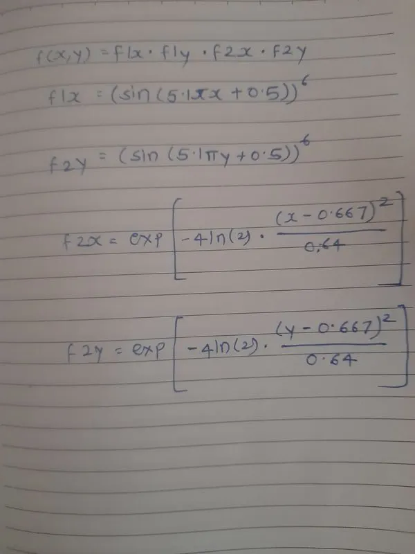
function [f]=stalagmite_function(input_vector)
x=input_vector(1);
y=input_vector(2);
f1=(sin(5.1*pi.*x+0.5)).^6;
f2=(sin(5.1*pi.*y+0.5)).^6;
f3=exp(-4*log(2).*(x-0.0667).^2/0.64);
f4=exp(-4*log(2).*(y-0.0667).^2/0.64);
f=-(f1.*f2.*f3.*f4);
end
Explanation:-
- Find out stalagmite Function used for loop
- defining x and y as inputs using linspace.
- loops are incorporated in main code so that all combinations of x and y values is taken in the stalagmite function.
- GA function runs for 50 iterations. plots of the stalagmite and maximum value generated in each iteration
- GA function is incorporated with lower and upper bounds and rns for 50 iterations.
Output:-