Week 4.1 - Genetic Algorithm

• Aim :-
• Write a code in MATLAB to optimise the stalagmite function and find the global maxima of the function.

• Objective :-
• Write a code in MATLAB to optimise the stalagmite function and find the global maxima of the function.
• Clearly expalin the concept of genetic algorithm in your own words and also explain the syntax for ga in MATLAB in your report.
• Make sure that your code gives the same output, even if it is made to run several times.
• Plot graphs for all 3 studies and for F maximum vs no. of iterations. Title and axes labels are a must, legends could be shown if necessary.

What Is the Genetic Algorithm?

The genetic algorithm is a method for solving both constrained and unconstrained optimization problems that is based on natural selection, the process that drives biological evolution. The genetic algorithm repeatedly modifies a population of individual solutions. At each step, the genetic algorithm selects individuals from the current population to be parents and uses them to produce the children for the next generation. Over successive generations, the population "evolves" toward an optimal solution. You can apply the genetic algorithm to solve a variety of optimization problems that are not well suited for standard optimization algorithms, including problems in which the objective function is discontinuous, non differentiable, stochastic, or highly nonlinear. The genetic algorithm can address problems of mixed integer programming, where some components are restricted to be integer-valued.

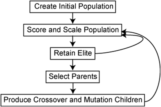
This flow chart outlines the main algorithmic steps.

The genetic algorithm uses three main types of rules at each step to create the next generation from the current population:

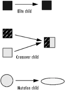
• Selection rules select the individuals, called parents, that contribute to the population at the next generation. The selection is generally stochastic, and can depend on the individuals' scores.
• Crossover rules combine two parents to form children for the next generation.
• Mutation rules apply random changes to individual parents to form children

The genetic algorithm differs from a classical, derivative-based, optimization algorithm in two main ways, as summarized in the following table:

Classical Algorithm	Genetic Algorithm
Generates a single point at each iteration. The sequence of points approaches an optimal solution.	Generates a population of points at each iteration. The best point in the population approaches an optimal solution.
Selects the next point in the sequence by a deterministic computation.	Selects the next population by computation which uses random number generators.
Typically converges quickly to a local solution.	Typically takes many function evaluations to converge. May or may not converge to a local or global minimum.

How the Genetic Algorithm Works

Outline of the Algorithm

The following outline summarizes how the genetic algorithm works:

1. The algorithm begins by creating a random initial population.
2. The algorithm then creates a sequence of new populations. At each step, the algorithm uses the individuals in the current generation to create the next population. To create the new population, the algorithm performs the following steps:
   1. Scores each member of the current population by computing its fitness value. These values are called the raw fitness scores.
   2. Scales the raw fitness scores to convert them into a more usable range of values. These scaled values are called expectation values.
   3. Selects members, called parents, based on their expectation.
   4. Some of the individuals in the current population that have lower fitness are chosen as elite. These elite individuals are passed to the next population.
   5. Produces children from the parents. Children are produced either by making random changes to a single parent—mutation—or by combining the vector entries of a pair of parents—crossover.
   6. Replaces the current population with the children to form the next generation.
3. The algorithm stops when one of the stopping criteria is met.
4. The algorithm takes modified steps for linear and integer constraints.
5. The algorithm is further modified for nonlinear constraints.

Introduction to stalagmites and stalactites function :-

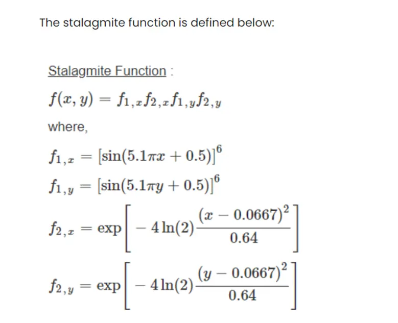
Stalactites are structures formed from mineral deposits that hang from caves. These formations hold tightly to the ceiling and hang down. Ad opposed to hanging from the ceiling stalagmite structures are formed from the cave floor that point upward. Stalagmite and stalactite function are mathematical function which represents shapes similar to that stalagmite and stalactites function.

Program for GA :-

close all
clear all
clc


x = linspace(0,0.6,150);
y = linspace(0,0.6,150);
limit = 30;

% Creating 2D array using meshgrid function
[xx,yy]= meshgrid(x,y);

% nested loop for array value input
for i=1:length(xx)
    for j=1:length(yy)
        input_vector(1)=xx(i,j);
        input_vector(2)=yy(i,j);
        f(i,j)= stalagmitefunc(input_vector);
    end
end
tic
for i = 1:limit
    [input,fval(i)]=ga(@stalagmitefunc,2);
    x_out(i)=input(1);
    y_out(i)=input(2);
end
case_time_1=toc;

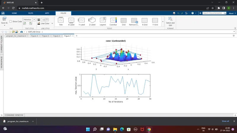
figure(1)
subplot(2,1,1)
surfc(xx,yy,-f)
xlabel('x')
ylabel('y')
title('case 1(unbounded)','color','k');
shading interp
hold on;
plot3(x_out,y_out,-fval,'marker','o','markersize',6,'MarkerFaceColor','r') 
subplot(2,1,2)
plot(-fval)
xlabel('No of Iterations')
ylabel('max. function value')

%case :2 Inserting Bounding Box
tic
for i=1:limit
    [input,fval(i)]=ga(@stalagmitefunc,2,[],[],[],[],[0;0],[0.6;0.6]);
    x_out(i)=input(1);
    y_out(i)=input(2);
end
case_time_2=toc;
figure(2);
subplot(2,1,1)
hold on;
surfc(xx,yy,-f)
xlabel('x')
ylabel('y')
title('case 2','color','k')
shading interp
plot3(x_out,y_out,-fval,'marker','o','MarkerSize',6,'markerfacecolor','y')
subplot(2,1,2)
plot(-fval)
xlabel('No of Iterations');
ylabel('max fuction value');

%case:3
options=optimoptions('ga');
options=optimoptions(options,'populationsize',100);
tic
for i=1:limit
    [input,fval(i)]=ga(@stalagmitefunc,2,[],[],[],[],[0,0],[0.6,0.6],[],[],options);
    x_out(i)=input(1);
    y_out(i)=input(2);
end
case_time_3=toc;
figure(3)
subplot(2,1,1)
hold on
surfc(xx,yy,-f)
shading interp
xlabel('x')
ylabel('y')
title('case 3','color','k')
plot3(x_out,y_out,-fval,'Marker','o','markersize',6,'markerfacecolor','y');
subplot(2,1,2)
plot(-fval)
xlabel('No of Iterations')
ylabel('max Function value')

%Case:4
options=optimoptions('ga');
options=optimoptions(options,'populationsize',300);

tic
for i =1:limit
    [input,fval(i)]=ga(@stalagmitefunc,2,[],[],[],[],[0,0],[0.1,0.1],[],[],options);
    x_out(i)=input(1);
    y_out(i)=input(2);
end
case_time_4=toc;
figure(4)
subplot(2,1,1)
hold on
surfc(xx,yy,-f)
shading interp
xlabel('x')
ylabel('y')
title('case 4','color','k')
plot3(x_out,y_out,-fval,'Marker','o','markersize',6,'MarkerFaceColor','r');
subplot(2,1,2)
plot(-fval)
xlabel('No of iteration')
ylabel('Max Function Value')
%Displaying the values of x and y for maximum value of function 
display(input)

%End of program


% Stalagmite function
function [f] = stalagmitefunc(input_vector)
f1x = (sin((5.1*pi).*input_vector(1)+0.5)).^6;
f1y = (sin((5.1*pi).*input_vector(2)+0.5)).^6;

f2x = exp((((input_vector(1)-0.0667).^2)/0.64).*(-4*log(2)));
f2y = exp((((input_vector(2)-0.0667).^2)/0.64).*(-4*log(2)));
f1 = f1x*f1y*f2x*f2y;
f = -f1;

end

Code Explanation :-

Firstly a random array of x and y vlues were creared and the corresponding 2D array was obtained using meshgrid function. A nested loop was used to assign values from this array into an array named input_vector is the input to the stalagmite function. The stalagmite function is written as separate. Minus (-) sign is given to the output of stalagmite function so that after the ga process it we get the blobal maxima (normally ga outputs global minima). Tic-toc command are used to get the running time of each case, in the first case the bounds were not defined and the plots were made. Negative sign is given for f value inside surface function to get the stalagmite function upwards. Bounding is given in next case so that the number of solutions approaches more accuracy. The population is increased in the subsequent cases and plotting is done,

The global maxima is found in the last case. The x and y values for which the function has maximum value is also displayed. The iterations were decreased to such a value that the results didn’t vary and the program consumed minimum time to execute.

Stopping Criteria :-

• Generation - The algorithm stops when the number of generations reaches the value of generations.
• Time limit – The algorithm stops after running for an amount of time in seconds equal to time limit.
• Fitness limit – The algorithm stops when the value of the fitness function for the best point in the current population is less than or equal to fitness limit.

Results -

Case 1 - Unbounded

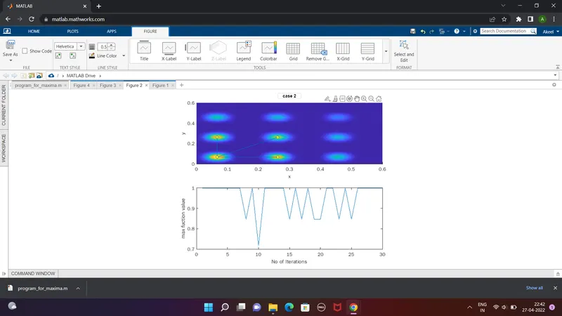
Case 2 - Bounded :-