Challenge

Week 3.5 - Deriving 4th order approximation of a 2nd order derivative using Taylor Table method

SSandeep Kolaparthi13 Jun 2022

MATLAB

Aim :

Derive the following 4th order approximations of the second-order derivative.

1. Central difference

2. Skewed right-sided difference

3. Skewed left-sided difference

Explanation :

1. Central Difference :

To derive central difference for fourth order approximation of second order derivative by taylor table method of finite difference method.

Second order derivative of fourth order approximation for CDS is :

f(x + ∆x) − 2f(x) + f(x − ∆x) ∆x2

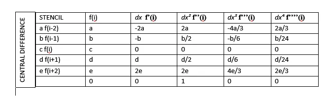
Central differences are useful in solving partial differential equations. If the data values are available both in the past and in the future, the numerical derivative should be approximated by the central difference.

Taylor table for central difference of fourth order approximation is :

Following MATLAB code written to find the value of above coefficients :

%Finding coefficients for above table

A = [ 1 1 1 1;-2 -1 0 1 2;2 0.5 0 0.5 2;-4/3, -1/6 0 1/6 4/3;2/3 1/24 0 1/24 2/3];

B = [0;0;1;0;0;]

C = inv(A)*B

Output : After solving the above matrix, we get values of all the coefficients :

a = -0.0833

b = 1.3333

c = -2.50

d = -1.333

e = -0.0833

Function for central difference 4th order error at particular spacing 'dx' :

function out = central_difference(x,dx)

% Function = exp(X)*cos(X);

%Analytical_derivative;

%second_order_analytical_derivative;

second_order_analytical_derivative = -2*sin(x)*exp(x);

%Fourth_order_approximation;

central_difference = (-0.0833*exp(x-2*dx)*cos(x-2*dx)+1.3333*exp(x-dx)*cos(x-dx)-2.50*exp(x)*cos(x)+1.3333*exp(x+dx)*cos(x+dx)-0.0833*exp(x+2*dx)*cos(x+2*dx))/dx^2;

out = abs(central_difference-second_order_analytical_derivative);

end

2. Skewed right-sided difference :

A right skewed distribution is sometimes called a positive skew distribution.

Taylor table for skewed right side difference of fourth order approximation :

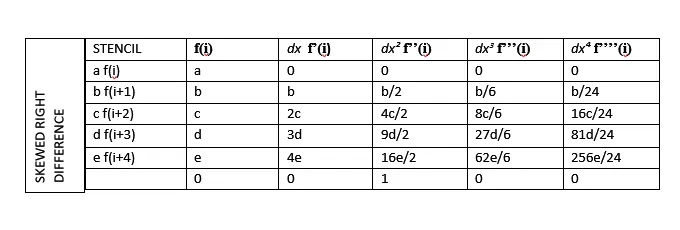
Following MATLAB code written to find the value of above coefficients :

%Finding coefficients for above table

A = [ 1 1 1 1 1;0 1 2 3 4;0 0.5 4/2 9/2 16/2;0 1/6 8/6 27/6 64/6; 0 1/24 16/24 81/24 256/24];

B = [0;0;1;0;0;]

C = inv(A)*B

Output : After solving the above matrix, we get values of all the coefficients :

a = 2.9166

b = -8.6666

c = 9.500

d = -4.666

e = 0.9166

Function for skewed right sided difference 4th order error at particular spacing 'dx' :

function out = skewed_right_side(x,dx)

%Function = exp(x)*cos(x);

%analytical_derivative;

%second_order_analytical_derivative;

second_order_analytical_derivative = -2*sin(x)*exp(x);

%Numerical_derivative;

%fourth_order_aproximation;

skewed_right_side = (2.9166*exp(x)*cos(x)-8.6666*exp(x+dx)*cos(x+dx)+9.500*exp(x+2*dx)*cos(x+2*dx)-4.666*exp(x+3*dx)*cos(x+3*dx)+0.9166*exp(x+4*dx)*cos(x+4*dx))/(dx^2);

out = abs(skewed_right_side-second_order_analytical_derivative);

end

3. Skewed left-sided difference :

Taylor table for skewed left side difference of fourth order approximation :

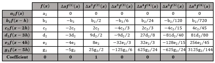
Following MATLAB code written to find the value of above coefficients :

%Finding coefficients for above table

A = [ 1 1 1 1 1;0 -1 -2 -3 -4;0 0.5 4/2 9/2 16/2;0 -1/6 -8/6 -27/6 -64/6; 0 1/24 16/24 81/24 256/24];

B = [0;0;1;0;0;]

C = inv(A)*B

Output : After solving the above matrix, we get values of all the coefficients :

a = 2.9166

b = -8.6666

c = 9.500

d = -4.666

e = 0.9166

Function for skewed left sided difference 4th order error at particular spacing 'dx' :

function out = skewed_left_side(x,dx)

%Function = exp(x)*cos(x);

%analyticl_derivative;

%second_order_analytical_derivative;

second_order_analytical_derivative = -2*sin(x)*exp(x);

%Numerical_derivative;

%Fourth_order_approximation;

skewed_left_side=(2.9166*exp(x)*cos(x)-8.6666*exp(x-dx)*cos(x-dx)+9.500*exp(x-2*dx)*cos(x-2*dx)-4.666*exp(x-3*dx)*cos(x-3*dx)+0.9166*exp(x-4*dx)*cos(x-4*dx))/dx^2;

out = abs(skewed_left_side-second_order_analytical_derivative);

end

Main Program :

clear all

close all

clc

%Input parameter

x=pi/3;

dx=linspace(pi/4,pi/4000,80);

%Function = exp(x)*cos(x);

%Analytical_derivative;

%second_order_analytical_derivative;

second_order_analytical_derivative = -2*sin(x)*exp(x);

%For loop

for i = 1:length(dx)

central_difference_error(i) = central_difference(x,dx(i));

skewed_right_side_error(i) = skewed_right_side(x,dx(i));

skewed_left_side_error(i) = skewed_left_side(x,dx(i));

end

%plotting;

figure(1)

loglog(dx,central_difference_error,'r','LineWidth',2)
hold on
grid on
loglog(dx,skewed_right_side_error,'g','LineWidth',2)
hold on
loglog(dx,skewed_left_side_error,'b','LineWidth',2)
%labelling;
xlabel('dx')
ylabel('error')
legend('central_difference_error','skewed_right_side_error','skewed_left_side_error')

Results :

Plot : Comparing absloute error of central difference with Skewed right-sided difference and Skewed left-sided difference

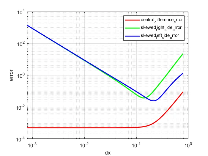
Conclusion : By the above plot we can conclude following observations which are as follows

Skewed right side diff gives max error and we can say that its unstable as compared to other scheme.
central difference gives lowest error and we can say that its stable as compared to other scheme.
skewed left sided diff gives error somewhere in between skewed right siide and central difference

Week 3.5 - Deriving 4th order approximation of a 2nd order derivative using Taylor Table method

Ship work like this
in your own course.

Talk to a career counsellor

Ship work like thisin your own course.

Talk to a career counsellor

Ship work like this
in your own course.