Week 4.1 - Genetic Algorithm
EXPLANATION OF THE CONCEPT OF GENETIC ALGORITHM:
The genetic algorithm reportadly modifies a population of individual solutions at each step, the genetic algorithm selects individual at random to the current position and uses them to produce the children for the next generation.
The genetic algorithm uses three main types of rules at each step to create the next generation from the current population
1.Selection rules select the individulas,called parents that contribute to the next generation.
2.Crossover rules combine two parents to form the next generation.
3.Mutation rules apply random changes to individual parents to form children.
SYNTAX OF 'GA'
x = ga(fun,nvars)
x= ga(fun,nvars,A,B)
x = ga(fun,nvars,A,B,Aeq,Beq)
x = ga(fun,nvars,A,B,Aeq,Beq,lb,ub)
x = ga(fun,nvars,A,B,Aeq,Beq,lb,ub,nonlocal)
x = ga(fun,nvars,A,B,Aeq,Beq,lb,ub,nonlocal,options)
x = ga(fun,nvars,A,B,Aeq,Beq,lb,ub,nonlocal,IntCon)
x = ga(fun,nvars,A,B,Aeq,Beq,lb,ub,nonlocal,IntCon,options)
x= ga(problems)
[x,fval] = ga(__)
[x,fval,exitflag,output]=ga(__)
[x,fval,exitflag,output,output,population,scores]=ga(__)
fitness fun fitness function
nvars number of design variables
Aineq A matrix for linear inequality comstraints
bineq B matrix for linear inequality constraints
Aeq Aeq for linear equality constraints
Beq Beq for linear eequality constraints
lb lower boundary of x
ub upper boundary of x
nonIcon nonlienear constraint function
rngstate optional state to reset the state of the random number generator
Solver 'ga'
options options created using optimotions or exported from the Optimization app
x = ga(fun,nvars) finds local unconstrained minimum x to the objective function fun nvars (number of design variables)
x= ga(fun,nvars,A,B) finds local maximum to the func,subject to the linear inequalities evaluates the matrix A*x and if x is transposed.
x = ga(fun,nvars,A,B,Aeq,Beq) finds local maximum to the func,subject to the linear Aeq*x = Beq inequalitiesA*x
x = ga(fun,nvars,A,B,Aeq,Beq,lb,ub) Designs a set of lower and upper bounds on the design vsrisbles so that the solutions is found in lb<x>ub
x = ga(fun,nvars,A,B,Aeq,Beq,lb,ub,nonlocal) subjects the minimisation of the constraints defined in non icon the function non icon accepts x and return vector covers c and ceq respresenting non linear inequalities and equalities.c(x),0
x = ga(fun,nvars,A,B,Aeq,Beq,lb,ub,nonlocal,options) minimises with default optimisation processes replaced by values in options nonlocal = [], create options using optimoptions.
x = ga(fun,nvars,A,B,Aeq,Beq,lb,ub,nonlocal,IntCon) requires that variales listed in intcon takes integer values.
x = ga(problem) finds minimum for the problem where problem is a structure.
[x,fval] =ga(__) for any previous input arguments also returns fval,the value of fitness function at x.
[x,fval,exitflag,output,output,population,scores]=ga(__)also returns a matrix population, whose rows are the final population,a vector scores, the scores of the final population.
Explanation of the code :
1. Firstly clear all the command window and figures by using clear all close all and clc.
2.Now define the workspace of x and y with 0 and 0.6 and number of elements has 150.
3.Creating the 2-Dimensional mesh by using the meshgrid command of x and y.
4.Now evaluate the stalagmite function by using the for loop of x and for loop of y and close both for loops.
5.Now use the surf command to create a graph, label the x and y axis with x data and y data.
6.For [inputs,fval] = ga(function,no of input variables) calls the output.
7.Now give the linspace of x and y with no of cases has 50
8.And create a for loop of x and y and give the inputs 1 and 2 and close the for loops.
9.For studying the statical behavaiour of maxima function,now use tic command it measures the elapsed time by using the toc command.
10.Now open the for loop for i = no of cases and output of[inputs,fopt(i)] = ga of stalagmite and no of varialbes has 2.
9.Since ga in a input varaible in stalagmite no need to mention it seperately in the function.
10.Now xopt and y opt has inputs,and close the function.
11.Take the study time has toc.
12.plot the figure(1) and subplot(2,1,1) and holdon surfc(x,y,-f) and plot xopt ,yopt,- fopt,marker,o,markersize,5,markerfacecolor,r)
13. give the title has Unbounded inputs and again subplot(2,1,2),plot(-fopt).
14. now label the x and y axis has iterations and function maximum.
15. Now studying the stastical behaviour with upper and lower bounds.
16.Open the for loop for i = no of cases and in the inputs of[inputs,fopt(i)] give ga(fun,nvars,A,B,Aeq,Beq,ub,lb) and xopt and yopt has inputs and end the for loop.
17.Now study time 2 same has that of the study time.
18. studying the increasing ga iterations.
19.Now use optimoptions commands which is used to return a list of options and defaults options for the default interior point in the fmicon algorithm optimoptions(options, population size,no of poplulations)
20.Now open the for loop of i = num of cases [inputs,fopt(i)]=ga(fun,nvars,A,B,Aeq,Beq,ub,lb,nonlocal,options) and give xopt and yopt of i has inputs of 1 and 2 respectively.
21.The plotting of the functions is same has that of the study time_2.
ERRORS FACED WHILE PROGRAMMING:
1.Inversion of the graph.
2.Execution of a script stalagmite has a function is not supported.
3.the line showing maxima curve is not appering.
STEPS TAKEN TO OVERCOME THESE ERRORS
1.We need to take function and fopt has negative.
2. Function name should be same in the ga while calling in all the three studies.
3.we need to give correct parenthesis for lower and upper bonds.
RESULTS :
The global maxima of the function is found.
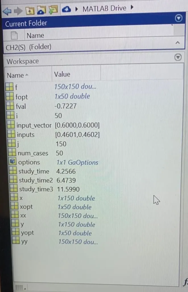
ERRORS:
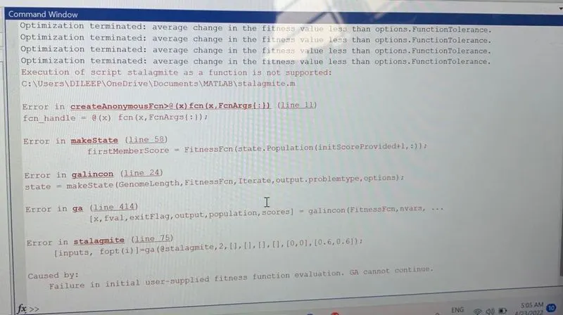
1 . Stalagmite:
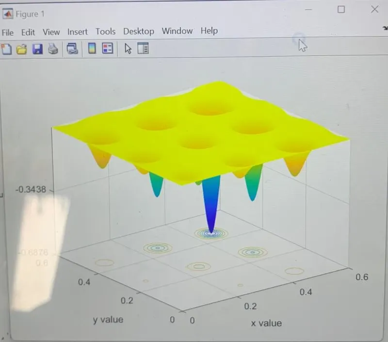
2. Unbounded inputs :
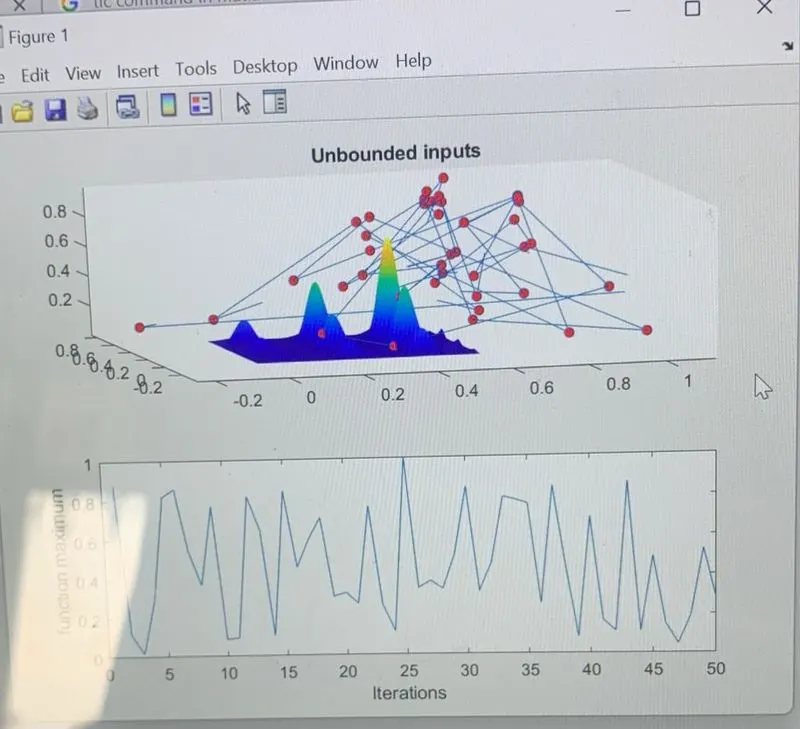
3. Lower and Upper boundes:
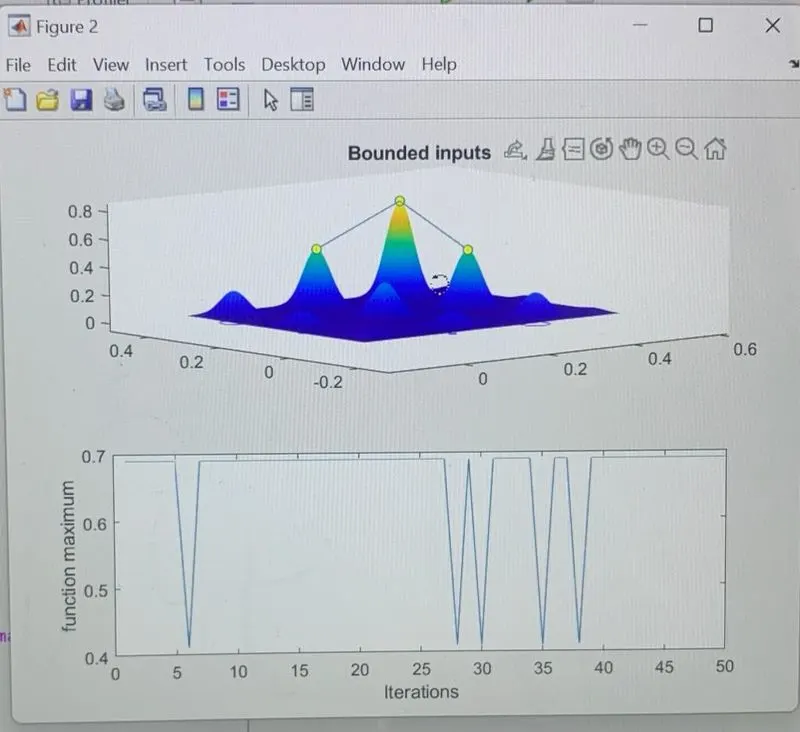
3. Bonded inputs with increasing population size :
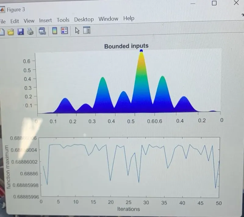
REFERENCES:
1. Genetic algorithm wikipedia.
clear all
close all
clc


% defining our search space
x = linspace(0,0.6,150);
y = linspace(0,0.6,150);

% creating 2Dimensional mesh
[xx, yy] = meshgrid(x, y);


% Evaluating the staglamite function
for  i = 1 : length(xx)
    for j = 1 : length(yy)
        input_vector(1) = xx(i,j);
        input_vector(2) = yy(i,j);
        f(i,j) = stalagmite_func(input_vector);
    end
end

surfc(xx,yy,f)
xlabel('x value')
ylabel('y value')

shading  interp

[inputs,fval] = ga(@stalagmite_func, 2);

%%


x = linspace(0,0.6,150);
y = linspace(0,0.6,150);
num_cases = 50;

for i = 1:length(x)
    for j = 1: length(y)
        inputs(1) = x(i);
        inputs(2) = y(j);
f(i,j) = stalagmite_func(inputs);
    end
end


%study 1 stastical behaviour

tic
for i = 1:num_cases
[inputs,fopt(i)] = ga(@stalagmite_func, 2);
xopt(i) = inputs(1);
yopt(i) = inputs(2);
end

study_time = toc;

%plotting
figure(1)
subplot(2,1,1);
hold on
surfc(x, y, -f)
shading interp
plot3(xopt,yopt,-fopt,'marker','o','markerSize',5,'markerfacecolor','r')
title('Unbounded inputs')
subplot(2,1,2)
plot(-fopt)
xlabel('Iterations')
xlabel('function maximum')

tic
 % study 2 - statistical behaviour - with upper amd lower bounds
 for i = 1:num_cases
     [inputs, fopt(i)]=ga(@stalagmite_func,2,[],[],[],[],[0,0],[1,1]);
     xopt(i) = inputs(1);
     yopt(i) = inputs(2);
 end

study_time2 = toc;

figure(2)
subplot(2,1,1)
hold on
surfc(x, y, -f)
shading interp
plot3(xopt,yopt,-fopt,'marker','o','markersize',5,'markerfacecolor','y')
title('Bounded inputs')
subplot(2,1,2)
plot(-fopt)
xlabel('Iterations')
xlabel('function maximum')


% study 3 increasing GA iterations
options = optimoptions('ga');
options = optimoptions(options,'populationSize',150);

tic
for i = 1:num_cases
    [inputs, fopt(i)]=ga(@stalagmite_func,2,[],[],[],[],[0,0],[1,1],[],[],options);
     xopt(i) = inputs(1);
     yopt(i) = inputs(2);
end

study_time3 = toc;

figure(3)
subplot(2,1,1)
hold on
surfc(x, y, -f)
shading interp
plot3(xopt,yopt,-fopt,'marker','o','markersize',5,'markerfacecolor','b')
title('Bounded inputs')
subplot(2,1,2)
plot(-fopt)
xlabel('Iterations')
xlabel('function maximum')


stalagmite function
function[stalagmite] = stalagmite_func(input_vector)

x = input_vector(1);
y = input_vector(2);

f1_x = (sin(5.1*pi*x+0.5)).^6;
f2_y = (sin(5.1*pi*y+0.5)).^6;
f3_x = exp((-4*0.693).*(x-0.667)^2/0.64);
f4_y = exp((-4*0.693).*(y-0.667)^2/0.64);
stalagmite = -(f1_x.*f2_y.*f3_x.*f4_y);
end