Week 4.1 - Genetic Algorithm

Aim: To find the global maxima on stalagmite function with the help of GA algarithm in Matlab

Objectives:

1. Write a code in MATLAB to optimise the stalagmite function and find the global maxima of the function.

2. Clearly expalin the concept of genetic algorithm in your own words and also explain the syntax for ga in MATLAB in your report.

3. Make sure that your code gives the same output, even if it is made to run several times.

4. Plot graphs for all 3 studies and for F maximum vs no. of iterations. Title and axes labels are a must, legends could be shown if necessary.

Theory :

1. Code in MATLAB to optimise the stalagmite function and find the global maxima of the function

Optimization concept:

Finding the approximate solution to a problem logically with out effecting the problem ,which otherwise takes life time to solve in treditional methods.By aproaching this method saves lot of time and investment.

Code:

%stalgamite function utilization to find the Global maxima
clear all
close all
clc

%inputs
x= linspace(0,0.6,150);  % using linspace command to create the 150 values between 0 to 0.6- to store in x variable
y= linspace(0,0.6,150);  % using linspace command to create the 150 values between 0 to 0.6- to store in y variable
num_cases=50;            % number of iterations = 50 
%2 Dimensional Mesh
[xx ,yy]= meshgrid(x,y); % meshing the x and y vectors  to create xx and yy mztrices.
%Evaluating the stalgamite functionclc
for i= 1:length(xx)      % creating for loop for xx values from 1 to no of values of xx
    for j=1: length(yy)  % creating for loop for xx values from 1 to no of values of yy
        input_vector(1)=xx(i,j); % xx points storing in a variable input_vector(1)
        input_vector(2)=yy(i,j); % yy points storing in a variable input_vector(1)
        f(i,j)=stalagmite(input_vector); % stalagmite function which is function of i,j
        %all created points from the loop are passed through the stalagmite
        %function.
    end
end
tic % Start stopwatch timer

surfc(x,y,-f)      %surface model display with x , y and -f 
hold on
%rng default;
xlabel('x values') %x-axis dispaly
ylabel('y values') %y-axis display
shading interp     %this command shades the graph to look smoother
%genetic algorithem with 2 variables x and y gives us out put of optimized x and y values(inputs) with respect to that fval(z value)
[inputs,fval]= ga(@stalagmite,2) 
Minimum = fval % randam  global minima(z value) displayed as minimum 

%case1: find the global maxima with out boundaries 
tic                                      %Start stopwatch timer
num_cases=50;                            %No of iterations are 50.
for i=1:num_cases                        % for loop to tun 50 times 
    [inputs,fout(i)]=ga(@stalagmite,2);  % inputs = Optimized x and y values & fout(i)= with reference to x & y finding  z value
    xout(i)=inputs(1);                   % inputs(1) are x values 
    yout(i)=inputs(2);                   % inputs (2) are y values
end
study1_time=toc;                         % toc is command to evaluate the time taking to tun the above iterations.
%plotting
figure(1)                                % image 1
subplot(2,1,1);                          % in the image 1 requires 2 rows and 1 coloumn and in that we are plotting at 1st row.
hold on                                  % continue display the same image window.
surfc(x,y,-f);                           % plotting the x ,y and f values to create the stalagmite surfaces
hold on                                  % continue display the same image window.
shading interp                           % this command shades the graph to look smoother
plot3(xout,yout,-fout,'marker','o','markersize',5,'markerfacecolor','r');
%ploting optimizes x , y , f values with circular marker of size 5 & color
%red.
title('unbounded inputs')                % title of the graph : unbounded inputs
subplot(2,1,2);                          % in the image 1 requires 2 rows and 1 coloumn and in that we are plotting at 2nd row.
plot(-fout);                             % plot the optimized values of f in the above specified location
xlabel('iterations')                     % x-axis : iterations
ylabel('optimized function value')       % y-axis: optimized function values(i.e.,z values)

%case2: finding the global maximum values randomly with boundary conditions
tic                                      % Start stopwatch timer               

 num_cases=50;                           % no of iterations: 50
for i=1:num_cases                        % i value = 1 to 50 nos.
    % below ga is from the syntax of ga- x = ga(fun,nvars,A,b,Aeq,beq,lb,ub)
    % fun= stalagmite function,nvars: 2 design variables (x & y)
    % A= Linear in equality constrains from real matrix
    % b= Linear in equality constrains from real vector
    % Aeq= Linear equality constrains from real matrix
    % beq= Linear equality constrains from real vector
    % as A,b,Aeq,beq are not available here we are keeping them as empty martix []
    [inputs,fout(i)]=ga(@stalagmite,2,[],[],[],[],[0;0],[0.6;0.6]); 
    xout(i)=inputs(1); % inputs(1) are  Optimized x values
    yout(i)=inputs(2); % inputs(2) are  Optimized y values
end
study_2=toc;           % toc is command to evaluate the time taking to tun the above iterations.
%plotting
figure(2)              % image 2
subplot(2,1,1);        % in the image 1 requires 2 rows and 1 coloumn and in that we are plotting at 1st row.
hold on                % stay on this image
surfc(x,y,-f);         % display the surface curve with x, y and f values 
shading interp         % this command is useful to smoothen the curve with out grids.
plot3(xout,yout,-fout,'marker','o','markersize',5,'markerfacecolor','r');
%ploting optimizes x , y , f values with circular marker of size 5 & color
title('bounded inputs')% title: bounded inputs.
subplot(2,1,2);        % in the image 1 requires 2 rows and 1 coloumn and in that we are plotting at 2nd row.
plot(-fout);           % plot the optimized values of f in the above specified location
xlabel('iteration')    % x-axis : iterations
ylabel('optimized function value') % y-axis : Optimized function values 

%case3:finding the global maximum values randomly with boundary conditions
%and also with population size 
options= optimoptions('ga');% this command defined the options from ga
options= optimoptions(options,'populationsize',170)% this command defines the population size (density of mesh)from options.
tic                    % Start stopwatch timer
 num_cases=50;         % no of iterations: 50 
for i=1:num_cases      % for loop runs 50 times 
    % below ga is from the syntax of ga- x =
    % ga(fun,nvars,A,b,[],[],lb,ub,nonlcon,IntCon,options)
    % fun= stalagmite function,nvars: 2 design variables (x & y)
    % A= Linear in equality constrains from real matrix
    % b= Linear in equality constrains from real vector
    % Aeq= Linear equality constrains from real matrix
    % beq= Linear equality constrains from real vector
    % nonlcon= non linear constrains 
    %Intcon= intiger variables
    % as A,b,Aeq,beq, nonlcon,Intcon are not available here we are keeping them as empty martix []
    [inputs,fout(i)]=ga(@stalagmite,2,[],[],[],[],[0;0],[0.6;0.6],[],[],options);
    xout(i)=inputs(1); % inputs(1) are  Optimized x values
    yout(i)=inputs(2); % inputs(2) are  Optimized y values
end
study_time3=toc;       % toc is command to evaluate the time taking to tun the above iterations.
figure(3)              % image 3
subplot(2,1,1);        % in the image 1 requires 2 rows and 1 coloumn and in that we are plotting at 1st row.
hold on                % stay on this image
surfc(x,y,-f);         % display the surface curve with x, y and f values
shading interp         % this command is useful to smoothen the curve with out grids.
plot3(xout,yout,-fout,'marker','o','markersize',5,'markerfacecolor','r');
%ploting optimizes x , y , f values with circular marker of size 5 & color
title('bounded inputs with modified population size') % title: bounded inputs.
subplot(2,1,2); % in the image 1 requires 2 rows and 1 coloumn and in that we are plotting at 2nd row.
plot(-fout);    % plot the optimized values of f in the above specified location
xlabel('iteration')                % x-axis : iterations
ylabel('optimized function value') % y-axis : Optimized function values

Code explanation :

Inorder to construct the stalagmite surface graph, we need mesh.

So, first constrcct the mesh surface-

by using linspace command we are taking different points of 150 Nos. between 0 to 0.6

in X-axis we are taking 150 data values & in y axis also we are taking 150 data values

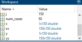
Now by using these values of x and y constructing the mesh with the help of mesh grid to get the points.

xx - points on x plain

yy- ponts on y plain

By considering each and every point on xx plain and also yy plain with the help of stalagmite function we will find the values on zz plain (optimised values).

stalagmite function:

%stalgamite function
function [f]= stalagmite(input_vector)
x= input_vector(1);
y= input_vector(2);

f1=(sin(5.1*pi*x+0.5))^6;
f2=(sin(5.1*pi*y+0.5))^6;
f3=exp(-4*log(2)*((x-0.0667)^2)/0.64);
f4=exp(-4*log(2)*((y-0.0667)^2)/0.64);
f=-(f1*f2*f3*f4);
end

This function find out the the optimised values by passing all the values of x and y through the equations f1,f2,f3,f4 as shown above and provides the value of 'f' which is optimised function value (z value) for each iteration or cycle.

so, as we are running this function 150 times with x values and 150 times with y values we will get different f values(say local minima if f is +ve & local maxima if f is -ve) for different x and y set of values.

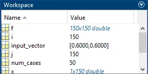
x values = i

y values = j as per above image.

so that all the grid points can be covered in the mesh.

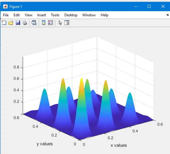
Now , with all the different values of obtained form a surface using surfc command

surfc(x,y,-f) to show the stalagmite graph as f is -ve it shows local maxima points.

using shading interp command grids can be avided in below image.

inputs(x and y values set) and fval(z value) randam points can be shown for every execution with the help of ga algorithm.

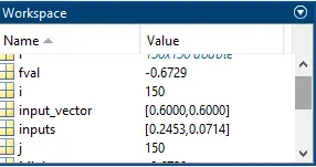
So, we can not find the global maxima at this level.as, here different optimal values comes for different executions and there so , here it is very critical to find the global maxima.

Study1: lets see by running the ga algorithm several times with out any boundary conditions.

This study gathers the number of optimized values (z values).

no of iterations =50 nos.

[inputs,fout(i)]=ga(@stalagmite,2);

xout(i)=inputs(1); = 50 values
yout(i)=inputs(2); = 50 values as shown below.

by looping the ga algorithm 50 times we will get 50 different optimised values .

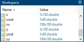
here fout optimised values 50 nos.

impose the optimised values on the stalagmite graph using marker command for understanding the random points.

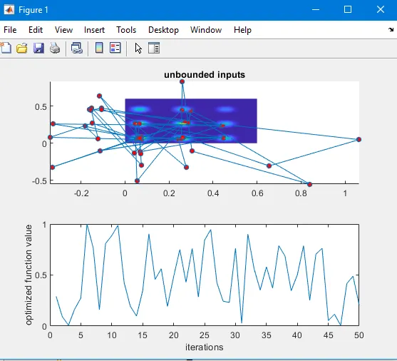
we can split the image with subplot(2(rows),1(column),1(1st row.) as shown above.

by seeing the above image we can understand that different random optimised points are selected and ploted with out any boundary constrains.

now plot fout values and see.

in the 2nd image (below) we can see the peaks and valleys of the values obtained due to randam optimised values.(fout)

In this condition also it is not that easy to find the global maxima value is difficult.

Study 2: By including the boundary conditions

In this case we will provide th eoundary condtions to the ga algorithm, so, optimised values can be defined with in these specified boundaries only.

below ga is from the syntax of ga- x = ga(fun,nvars,A,b,Aeq,beq,lb,ub)
fun= stalagmite function,nvars: 2 design variables (x & y)
A Linear in equality constrains from real matrix
b= Linear in equality constrains from real vector
Aeq= Linear equality constrains from real matrix
beq= Linear equality constrains from real vector
as A,b,Aeq,beq are not available here we are keeping them as empty martix []

[inputs,fout(i)]=ga(@stalagmite,2,[],[],[],[],[0;0],[0.6;0.6]);

here boundary condtions are 0.6 on x axis and 0.6 on y axis.

By considering the optimised values from previous case.run this algorithm for 50 iterations to provide the optimal values for 50 cycles.

and result shows the few points of optimised with in the boundaries of 0.6 x axis and 0.6 y axis.

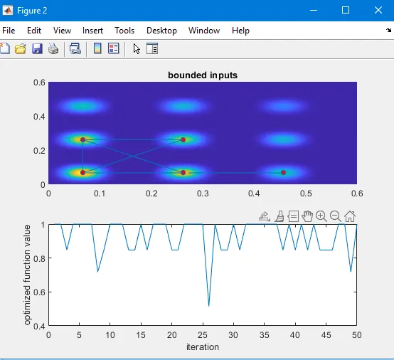
Here also it difficult to find out the single value of global maxima.

Study3:By concentrating on population size (grid size on the graph) to obtain the best values.

for 50 iterations of the ga algorithm with population size shown as below.

[inputs,fout(i)]=ga(@stalagmite,2,[],[],[],[],[0;0],[0.6;0.6],[],[],options);

Above ga is from the syntax -
ga(fun,nvars,A,b,[],[],lb,ub,nonlcon,IntCon,options)
fun= stalagmite function,nvars: 2 design variables (x & y)
A= Linear in equality constrains from real matrix
b= Linear in equality constrains from real vector
Aeq= Linear equality constrains from real matrix
beq= Linear equality constrains from real vector
nonlcon= non linear constrains
Intcon= intiger variables
as A,b,Aeq,beq, nonlcon,Intcon are not available here we are keeping them as empty martix []

Here Options are population sizes

options= optimoptions('ga');

by using optimoptions command declaring 'ga' as solver

now decalring the population size as 170

options= optimoptions(options,'populationsize',170)

now plot the optimised points and fout values to get the global maxima.

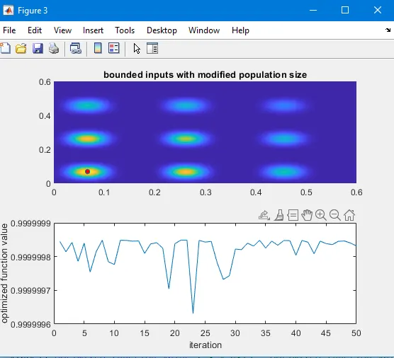
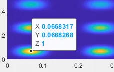
This graph clearly explains with marker that the higlighted point is global maxima.

and 2nd graph shows the value of the fout (global maxima ie., z value)= near to the 0.9999996

xout values =

yout values =

fout values=

______________________________________________________________________________

2.Genetic Algorithm (GA):

As the name Genetic indicates the genuie related concept.This algorithm is a gentic way of solving the problems to get the optimised solution.

Steps in GA :

1. Considering the initial data with out any limts or boundaries or constrians.With the help of fitness function select the best fitting data based on fitness( data which are showing the local minima )of the data.

2. These slected data under goes for Cross over process, in these data values which gives lowest values are a said to be equating the genes and produces the next generation points .

3. These points under goes mutaion process to interchange the genes and produces the better optimised data values .

Syntax:GA

There are several syntax for GA at different conditions .

Out of this we are using 3 syntaxes

1. x = ga(fun,nvars)

This is using when we are having only fitness function and design variables to solve the problem.

2.x= ga(fun,nvars,A,b,Aeq,beq,lb,ub)

This is using when we are having the fitness function, design variables,linear inequality constrians in matrices,linear in equality constrains in real vectors,Equality constrains in matrices,equality constrains in vectors,lower boundaries ,upper boundaries are avaialable to solve the problem.

3. x= ga(fun,nvars,A,b,[],[],,lb,ub,nonlcon,IntCon,options)

This is using when we are having the fitness function, design variables,linear inequality constrians in matrices,linear in equality constrains in real vectors, No -Equality constrains in matrices, No -equality constrains in vectors,lower boundaries ,upper boundaries,Non linear constrains, Intiger values,Optimization options(population size) are avaialable to solve the problem.