Week 3 - Solving second order ODEs
INTRODUCTION:
In Engineering, Ordinary Differential Equation is used to describe the transient behavior of a system. Hence pendulum is considered .
The way the pendulum moves depends on the Newtons second law. When this law is written down, we get a second order Ordinary Differential Equation that describes the position of the "ball" w.r.t time.
OBJECTIVE:
The bjective is to write a program that solves the ODE that represents the equation of motion of a simple pendulum with damping
Second Order ODE:
This equation derived from the Newtons 2nd law of motion :
`(d^2theta)/dt^2 + b/m* (d theta)/dt + g/l* sin theta = 0`
In the above equation,
g = gravity in m/s2,
L = length of the pendulum in m,
m = mass of the ball in kg,
b=damping coefficient.
ODE MATRICES :
if `theta = theta1`
`(d^2theta1)/dt^2 + b/m* (d theta1)/dt + g/l* sin theta1 = 0`
`(d theta1)/dt =theta2` ---- Equation 1
`(d theta2)/dt = - b/m* theta2 - g/l* sin theta1`
`d/dt[(theta1),(theta2)] = [(theta2),(-b/m*theta2-g/l*sintheta1)]`
`(d theta)/dt = [(theta2),(-b/m*theta2-g/l*sintheta1)]` ---- Equation 2
theta2 = angular displacement
-b/m*theta2-g/l*sintheta1 = angular velocity
PROGRAM TO SIMULATE THE MOTION OF SIMPLE PENDULUM:
%program to solve 2nd order ODE to simulate the simple pendulam
clear all
close all
clc
% formula retrived from the newtons seond law : d^2theta_dt^2+(b/m)*d^theta_dt+(g/l)*sind(theta)

%input values
b=0.05;                       %damping co-efficient
m=1;                          %ball mass in kg
g=9.8;                        %gravity in m/sec^2
l=1;                          %length of the string
%initial condition
theta_0=[0;3]                 %initial displacment;initial angular velocity in radians

%time
time_span=linspace(0,20,500); %duration of motion

%solve ODE by using ode45 solver
%anonymus function inputs t and theta
[t,results]=ode45(@(t,theta)ode_func(t,theta,b,g,l,m),time_span,theta_0);
figure(1)                     %result window 1
plot(t,results(:,1));         %print the angular displacement values
hold on                       %stay in the same graph
plot(t,results(:,2));         %print the angular velocity values
ylabel('position')            %position
xlabel('time')                %time
grid on;

theta2 =results(:,1)          %angular dispalcement:  theta2

ct=1;
for i=1:length(theta2);       %for loop from 1 to change in displacement values

    theta_temp= theta2(i);    %create temperarory variable

    x0=0;                     %1st x  co ordinate of the string
    y0=0;                     %1st y  co ordinate of the string
    x1=l*sin(theta_temp);     %2nd x  co ordinate of the string
    y1=-l*cos(theta_temp);    %2nd y  co ordinate of the string
    figure(2)                 %result window 2
    plot([-0.5 0.5],[0 0],'linewidth',5); %print a line on x axis
    hold on;                              %hold it on same window
    plot([x0 x1],[y0 y1],'linewidth',3);  %print a line with co-ordinates x0,y0 and x1,y1 to get string
    hold on;                              %hold it on same window
    plot(x1,y1,'o','markers',15,'markerfacecolor','g') %print the string along with a ball marker of size 15 & green colour
    hold off                                           %don't hold the picture
    grid on                                            %grid on
    axis ([-1.5 1.5 -1.5 0.5]);                        %setting axis position
    pause(0.002)                                       %pause for every 0.002 seconds
    M(ct)= getframe(gcf);                              %vaiable to store the video
    ct=ct+1;                                           %increment
end
movie(M)                                               % create movie with variable M
videofile= VideoWriter('pendulum.avi','Uncompressed avi'); % write the video in to avi format
open(videofile)                                            %open the video
writeVideo(videofile,M)                                    %write the video from vaiable M
close(videofile)                                           %close the video
STEP WISE EXPLANATION OF CODE:
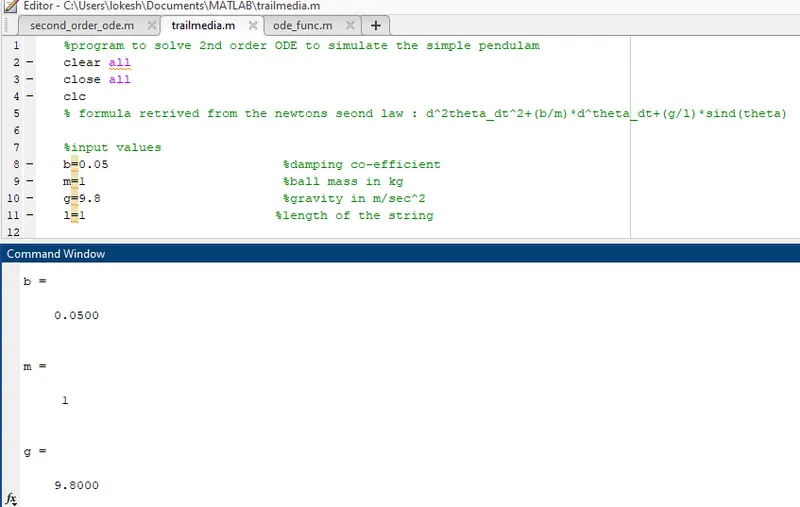
Step1: Considering the given inputs
damping co-efficient(b) = 0.05
mass of the ball (m) = 1 kg
gravity (g) = 9.8 m/sec
length of the string (l) = 1 meter
results:
____________________________________________________
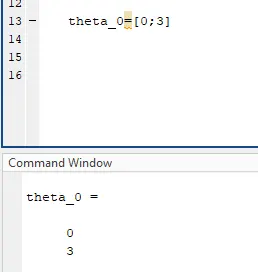
Step2: Initial conditions
from Equation 2:
theta_0=[angular displacement;angular velocity]
hence,
Initial angular dispalcement = 0
Initial angular velocity = 3
results:
_________________________________________________
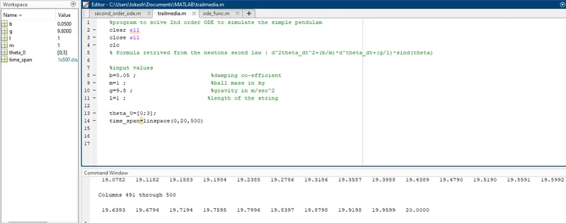
step3: Pendulum motion time
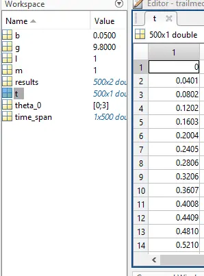
time_span=0 to 20 sec 500 values by using the linspace command
linspace(0,20,500)
results:
______________________________________________________________
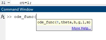
step4: engaging the ODE 45 function solver to solve 2nd order ODE
[t,results]=ode45(@(t,theta)ode_func(t,theta,b,g,l,m),time_span,theta_0);
inputs = t & theta
function :ode_func(t,theta,b,g,l,m)
t = time
theta = theta
time_span = motion time
theta_0 = initial conditions
function [dtheta_dt]= ode_func(t,theta,b,g,l,m) %function variables
theta1=theta(1);                            %theta1
theta2=theta(2);                            %theta2

dtheta1_dt=theta2;                          %angular displacement
dtheta2_dt=-(b/m)*theta2-(g/l)*sin(theta1); %angular velocity
dtheta_dt=[dtheta1_dt;dtheta2_dt];
end
results:
__________________________________________________________
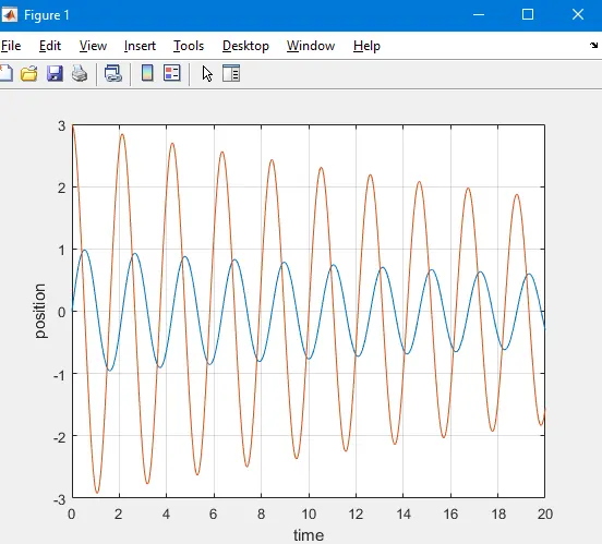
step5: plotting the results of angular displacement
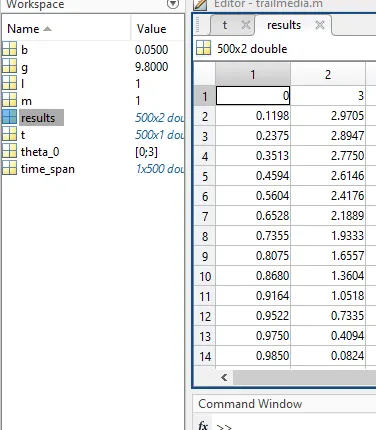
plot(t,results(:,1)); - vector matrics of results with respect to the time with the help of ode45 solver
and assign the variable theta2 = results(:,1)
step6: plotting the results of angular velocity
plot(t,results(:,2)); - vector matrics of reults with respect to the time with the help of ode45 solver.
results of time :
results angular dispacement and angular velocity:
results showing the damping varaition of anglar dispalcement as well as angular velocity with respect to the time:
step7:for loop from 1 to up to the length of theta2 i.e., all angular dispalcment values with repect to the different timings
intial co ordinates x0,y0=0,0
theta_temp =theta2(i) temporary variable
x1= l*sin(theta_temp); x corodinate
y1=-l*cos(theta_temp); y coordinate with negative sign to show downwards
figure(2) second window
plot([-0.5 0.5],[0 0],'linewidth',5); printing the horizontal line as a hinge 0.5 mm away from center.
hold on; to stay on same window
plot([x0 x1],[y0 y1],'linewidth',3); printing the string line with respect to the co ordinates.
hold on ; to saty on same window
plot(x1,y1,'o','markers',15,'markerfacecolor','g'; to print the pendulum bob using the 'o' marker with size 15 and green colour
hold off; to mantian single image
pause ; to hold them for 0.002 sec every picture
M(ct)= getframe(gcf) ; getting the current frame and feed in to the variable M
end of the loop
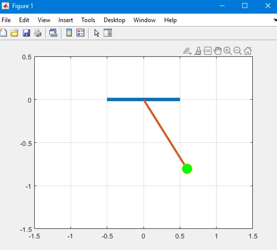
_____________________________________________________________
step8:creating the animation
making a movie -
movie(M) %to create movie with variable M
videofile= VideoWriter('pendulum.avi','Uncompressed avi');
% write the video in to avi format
open(videofile) %open the video
writeVideo(videofile,M) %write the video from vaiable M
close(videofile) % close the video file.
Errors:
1.Error1:

Mistake:

I used marker as command instead of markers
Corrective action:

2.Error2:
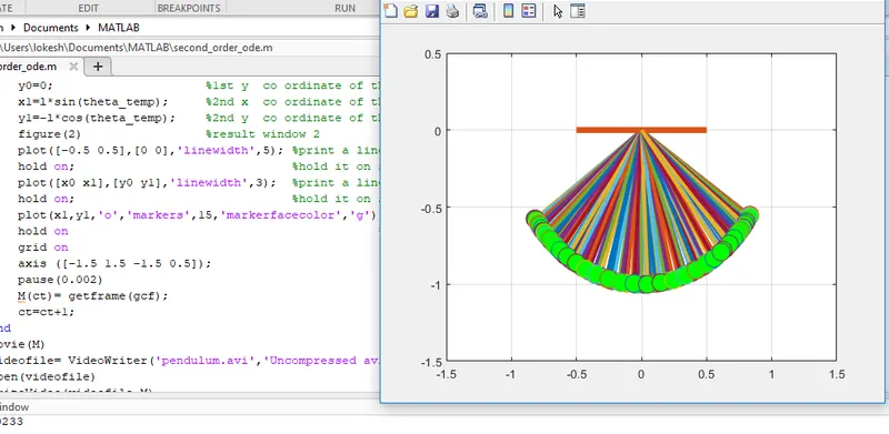
Mistake:

corrective action:

Youtube link for animation:
https://youtu.be/SMyl_YG3QK0