Analysis of P.V Diagram and Thermal efficiency on Otto cycle using matlab

Project objective: To create the pressure and volume diagram and find the thermal efficiency of an otto cycle engine using matlab program.

Theory: Theory behind the otto cycle is as below-

Otto cycle is an ideal engine cycle which explains the concept of reciprocating phenomena of the engine parts which leads to the power generation ultimately.

Process1: Isentropic compression means Iso +entropy

Iso - common

Entropy - it is a unit which explains the change in thermal energy in the system to other form of energy.

Adiabatic compression of ideal gas - p.v ^γ = constant

At stage 1:

Pressure p1

Temperature t1

Volume v1

When piston moves from BDC to TDC (crank angle 180 to 360) it is called compression process

During this process moves to stage 2

Stage 2:

Pressure p2

Temperature t2

Volume v2

Now, volume remains constant as the piston remains rest at this process.

In this stage 3:

Combustion occurs and so,

Temperature increases to t3

Pressure increases to p2

But volume remains same v3 =v2

Now, piston moves down with the power gain so,

At this stage 4:

Expansion occurs so,

Volume changes to normal = v4 =v1

Temperature reduces= T4

Pressure changes =p4

Otto cycle program coding:

%otto cycle main program
clear all
close all
clc

%inputs
gama=1.4;
t3=2300;%kelvins

%state variables
p1=103125;%pascals
t1=500;%kelvins

%engine geometric parameters
bore=0.1; %meter
stroke=0.1;%meter
con_rod=0.15;%meter
cr=12;

%Calculating swept volume and clearence volume
v_swept=(pi/4)*bore^2*stroke;
v_clr=v_swept/(cr-1);


v1=v_swept+v_clr ;                  %step1
v2=v_clr;

%state variables at state point2
%p1v1^gama=p2v2^gama
%p2=p1v1/v2^gama =p1cr^gama
p2=p1*cr^gama;
%p1v1/t1=p2v2/t2
t2=p2*v2*t1/(p1*v1);                %step2

%step7:
constant_c=p1*v1^gama;
v_compression=engine_kinematics2(bore,stroke,con_rod,cr,180,0);
p_compression=constant_c./v_compression.^gama;


%state variables at state point 3
v3= v2;
%p3v3/t3=p2v2/t2
%p3=p2*v2*t3/(v3*t2)
p3=(p2*t3)/t2;                      %step3


%step7:
constant_c=p3*v3^gama;%isentropic expansion constant=p*v^gama
v_expansion=engine_kinematics2(bore,stroke,con_rod,cr,0,180);
p_expansion=constant_c./v_expansion.^gama;

%state variables at state point4
v4=v1;

%p3v3^gama=p4v4^gama;
p4=p3*(v3/v4)^gama ;                %step4

figure(1)                          %function variable 
hold on

plot(v1,p1,'*','color','r')        % to print (v1,p1) point (step5)
plot(v_compression,p_compression)  %step8 explains
plot(v2,p2,'*','color','r')        % to print (v12,p2) point(step5)
plot([v2 v3],[p2 p3],'color','b')  %step9 explains
plot(v3,p3,'*','color','r')        % to print (v3,p3) point(step5)
plot(v_expansion,p_expansion)      % step 8 explains
plot(v4,p4,'*','color','r')        % to print (v4,p4) point(step5)
plot([v4 v1],[p4 p1],'color','b')  %step9 explains

%tep10:
eta=1-(1/cr^(gama-1));
thermal_efficeincy_of_engine = eta*100

______________________________________________________________

Function program coding:

%program for function 
function [v]= engine_kinematics2(bore,stroke,con_rod,cr,start_crank,end_crank)




a=stroke/2;
R=con_rod/a;

v_swept=(pi/4)*bore^2*stroke;
v_clr=v_swept/(cr-1);

theta=linspace(start_crank,end_crank,179);

term1=0.5*(cr-1);
term2=R+1-cosd(theta);
term3=(R^2-sind(theta).^2).^0.5;

%step6:

v= (1+term1*(term2-term3)).*v_clr;

end

__________________________________________________________

Explanation of program:

Step1:

We have to calculate the stage position points of pressure and volume ie., v1,v2,v3,v4,p1,p2,p3,p4

Inputs : pressure p1 = 101325 Pascal’s , temperature t1 = 500 kelvins , γ =1.4, t3 =2030 kelvins

To calculate v1:

v1 describes the location of piston in the BDC of the engine.

Geometric parameters of the engine:

Bore = 0.1 meter

Stroke = 0.1 meter

Connecting rod length - 0.15 meter

Compression ratio (cr) = 12

Swept volume =

Clearance volume= =v2

v1 = swept volume + clearance volume

Output at step1:

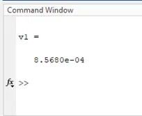
step2: Calculating at stage 2:

Isentropic compression

…………………………….calculated

now combined gas law- p1*v1/t1=p2*v2/t2

t2 = p2*v2*t1 /(p1*v1)……………………calculated

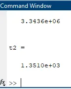
Output at step2:

&

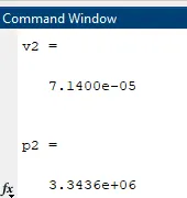step3: at stage 3-

v3 = v2 as it is constant volume heat addition stage

t3 is input

Calculating p3-

As per combined gas law p2*v2/t2 = p3*v3/t3

Hence p3 = p2*t3/t2 (as volumes get cancelled)……..calculated

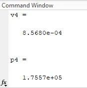
Output at step3:

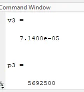
Step4:

Isentropic expansion-

Isentropic compression

V4 =v1

…………………………….calculated

Output at step4:

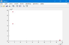
Step5:

Now plot the volumes and pressures at different stages

Plotting individual volume and pressure variables set at each stage in a single window by using

Figure command.

Output at step5:

Step6:

In order to get the traceability of variables in isentropic compression and isentropic expansion process

Enclose the function program of engine kinematics:

Inputs:

Geometric parameters of the engine specified above.

Function [v] = engine_kinematics(bore,stroke,con_rod,cr,start_crank,end_crank)

By using the formula of volume traceability derived from purely geometrical relationship-

R = connecting rod length/a

a = stroke/2

in order to make it easy divide the formula in to terms

find the value of v by using above formula

make the theta as matrix using linspace command

Input at step6:

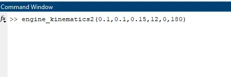
Output at step6:

step7:

Incorporate the function in to the regular program-

Use the function ‘engine_kinematics ‘ at compression stage by calculating v-compression variable

As it is a isentropic process

And give start _crank =180 end_crank=0 in function variable

To find v_ compression…………….calculated

Use the function ‘engine_kinematics ‘ at expansion stage by calculating v-expansion variable

As it is a isentropic process

And give start _crank =0 end_crank= 180 in function variable

To find v_ expansion…………….calculated

Step8:

Plotting the volume and pressure variables at compression stage ie., v_compression & p_compression after stage 2

Plotting the volume and pressure variables at compression stage ie., v_expansion & p_expansion after stage 3

Output at step8:

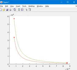
Step9:

Add the variables of stage 2 and stage 3 in a vector matrix i.e., [v2 v3],[p2 p3] in the plot command

By providing colour to them

As well as add the variables of stage 4 and stage 1 in a vector matrix i.e., [v4 v1],[p4 p1] in the plot command by providing colour to them

Output at step9:

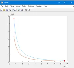
Step10:

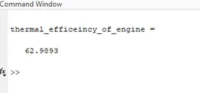
Calculating thermal efficiency of the engine-

Formula= (eta)

% of the efficiency = eta*100

Outputs at step10:

_____________________________________________________________________

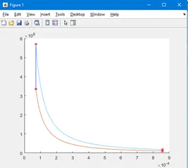
Errors:

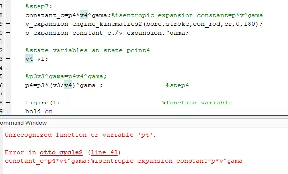
Solution for error:

Error resolved