Week 4.1 - Genetic Algorithm
Stalagmite Mathematical Model
AIM: Write a code to optimize the stalagmite function and find the global maxima of the function
OBJECTIVES:
- To write a code in MATLAB to optimize the stalagmite function and find the global maxima of the function
- To explain the concept of genetic algorithm and its syntax
- To plot graphs for all three studies and for F maximum vs number of iterations
THEORY:
Genetic algorithm: It is a search heuristic and optimization algorithm which is inspired by Charles Darwin’s theory of natural evolution. This algorithm shows the process of natural selection from the generation where the fittest individuals are selected from the generation for the reproduction to produce offspring of the next generation, the fittest ones will survive in the next generation. Genetic algorithms imitate the process of natural selection.
There are 5 phases in genetic algorithm which are as follows:
- Initial population
- Fitness function
- Selection
- Crossover
- Mutation
Syntax of ga:
X = ga (fitnessfcn, nvars, Aineq, bineq, Aeq, beq, lb, ub, nonlcon, intcon, options)
Where,
fitnessfcn: Fitness function
nvars: Number of design variables
Aineq: A matrix for inequality constraints
bineq: b vector for inequality constraints
Aeq: Aeq matrix for equality constraints
beq: beq vector for equality constraints
lb: Lower bound on X
ub: Upper bound on X
nonlcon: Nonlinear constraint function
intcon: Index vector for integer variables
options: Options created with optimoptions('ga')
FLOWCHART:
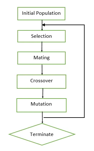
- The evolution usually starts from a population of randomly generated individuals
- Individual solutions are selected through a fitness-based process
- This generation process is repeated until a termination condition has been reached
- Improve the solution through repetitive application of the selection, crossover, and mutation operators
BODY OF THE CONTENT:
Programming language: MATLAB
Code:
Global optimization of stalagmite function and finding global maxima
% Global Optimization of stalagmite function
close all
clear all
clc

% Defining our search space
x = linspace(0,0.6,150);
y = linspace(0,0.6,150);

% Creating a 2-Dimensional mesh
[xx, yy] = meshgrid(x,y);

% Evaluating the stalagmite function
for i = 1:length(xx)
    for j = 1:length(yy)
        input_vector(1) = xx(i,j);
        input_vector(2) = yy(i,j);
        f(i,j) = stalagmite(input_vector);
    end
end

% Plotting
surfc(xx,yy,f)      % 3D visualization of function
xlabel('x axis')
ylabel('y axis')
zlabel('z axis')
title('Stalagmite function visualization')
shading interp      % removes grid lines

% Using Genetic algorithm for evaluating optimum value
[inputs, fval] = ga(@stalagmite, 2)
- First we define search space by defining variables x and y and initializing them with the linear array
- Then we use meshgrid command to create 2Dimensional array
- Then we use nested for loop to initialize input vector and call stalagmite function
- surfc command is used to plot the function for visualization and use shading interp command to hide gridlines
- Then we use ga function to evaluate optimum value of stalagmite function
Stalagmite function
% Stalagmite function
function [f] = stalagmite(input_vector)

x = input_vector(1);
y = input_vector(2);

f1 = (sin(5.1*pi*x + 0.5))^6;
f2 = exp(-4*log(2)*((x-0.0667)^2)/0.64);
f3 = (sin(5.1*pi*y + 0.5))^6;
f4 = exp(-4*log(2)*((y-0.0667)^2)/0.64);
f = -(f1*f2*f3*f4);
end- Code for stalagmite function, in this code stalagmite function expressions are solved and stored in variable f
Statistical Behavior
% Statistical behavior

clear all
close all
clc

x = linspace(0,0.6,150);
y = linspace(0,0.6,150);

% Creating a 2-Dimensional mesh
[x,y] = meshgrid(x,y);
% Defining number of iterations
num_cases = 50;
% Calling get_stalagmite function
f = get_stalagmite(x,y);


% Study 1: Statistical behavior
tic    % Timer
for i = 1:num_cases
    [inputs, fopt(i)] = ga(@stalagmite,2);  % Calling ga function
    xopt(i) = inputs(1);
    yopt(i) = inputs(2);
end
study1_time = toc

figure(1)
subplot(2,1,1)
hold on
surfc(x, y, f)
shading interp
plot3(xopt, yopt, fopt,'marker','o','markersize', 5,'markerfacecolor','r')
title('Unbounded inputs')

subplot(2,1,2)
plot(fopt)
xlabel('Iterations')
ylabel('Function minimum')
title('Statistical behavior')

% Study 2: Statistical behavior - with upper and lower bounds
tic     % Timer
for i = 1:num_cases
    [inputs, fopt(i)] = ga(@stalagmite,2,[],[],[],[],[0,0],[1,1]);
    xopt(i) = inputs(1);
    yopt(i) = inputs(2);
end
study2_time = toc

figure(2)
subplot(2,1,1)
hold on
surfc(x, y, f)
shading interp
plot3(xopt, yopt, fopt,'marker','o','markersize', 5,'markerfacecolor','r')
title('Bounded inputs')
subplot(2,1,2)
plot(fopt)
xlabel('Iterations')
ylabel('Function minimum')
title('Statistical behavior')

% Study 3: Statistical behavior - increasing ga iterations
options = optimoptions('ga');
options = optimoptions(options,'PopulationSize',170);   % Increasing iterations

tic     % Timer
for i = 1:num_cases
    [inputs, fopt(i)] = ga(@stalagmite,2,[],[],[],[],[0,0],[1,1],[],[],options);
    xopt(i) = inputs(1);
    yopt(i) = inputs(2);
end
study3_time = toc

figure(3)
subplot(2,1,1)
hold on
surfc(x, y, f)
shading interp
plot3(xopt, yopt, fopt,'marker','o','markersize', 5,'markerfacecolor','r')
title('Bounded inputs with modified population size')
subplot(2,1,2)
plot(fopt)
xlabel('Iterations')
ylabel('Function minimum')
title('Statistical behavior')- In this code there are three studies for analyzing the genetic algorithm to determine the optimum value
- First we define search space by defining variables x and y and initializing them with the linear array
- Then we use meshgrid command to create 2Dimensional array
- Number of iterations is defined and get stalagmite function is called, which gives matrix f
- In first study the ga function is used where syntax has only number of variables, which gives a unbounded inputs values
- Second study involves the use of ga function with syntax having the upper and lower bounds so that the results are contained within a specified bonds
- Third study uses ga function with syntax additionaly having options which is used to increase the population size
- Figures of all three studies are plotted and the difference of time taken to run all the three studies is observed
get_stalagmite function code
% get_stalagmite function

function [f] = get_stalagmite(x,y)


f1 = (sin(5.1*pi.*x + 0.5)).^6;
f2 = exp(-4*log(2).*((x-0.0667).^2)/0.64);
f3 = (sin(5.1*pi.*y + 0.5)).^6;
f4 = exp(-4*log(2).*((y-0.0667).^2)/0.64);
f = -(f1.*f2.*f3.*f4);
end- Code for get stalagmite function, in this code stalagmite function expressions are solved and stored in variable f
ERRORS:
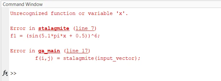
- This error was in the function tempate of stalagmite, it was due to not defining the variables x and y
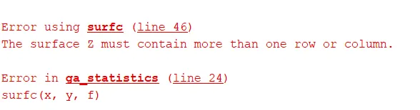
- This error occured due to mismatching of the matrix size while executing the surfc command to plot, it was due to not using the meshgrid command
RESULTS:
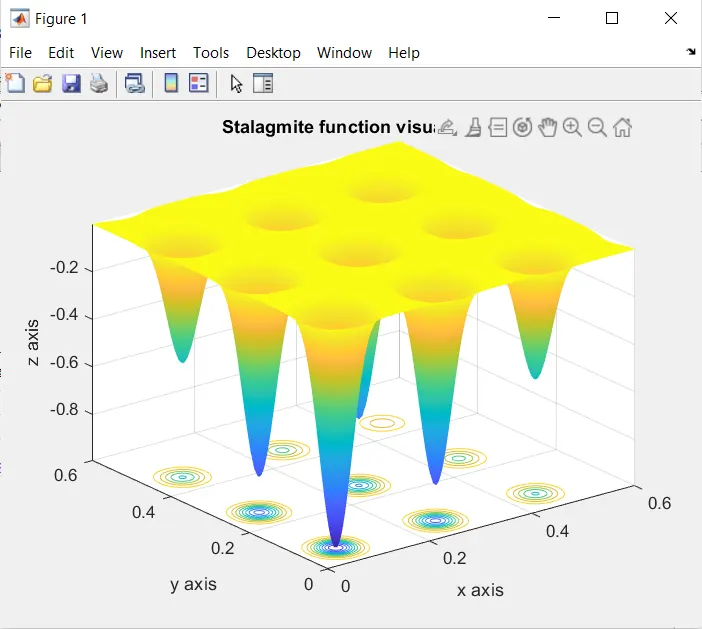
- The above figure shows the 3D visualization of stalagmite function
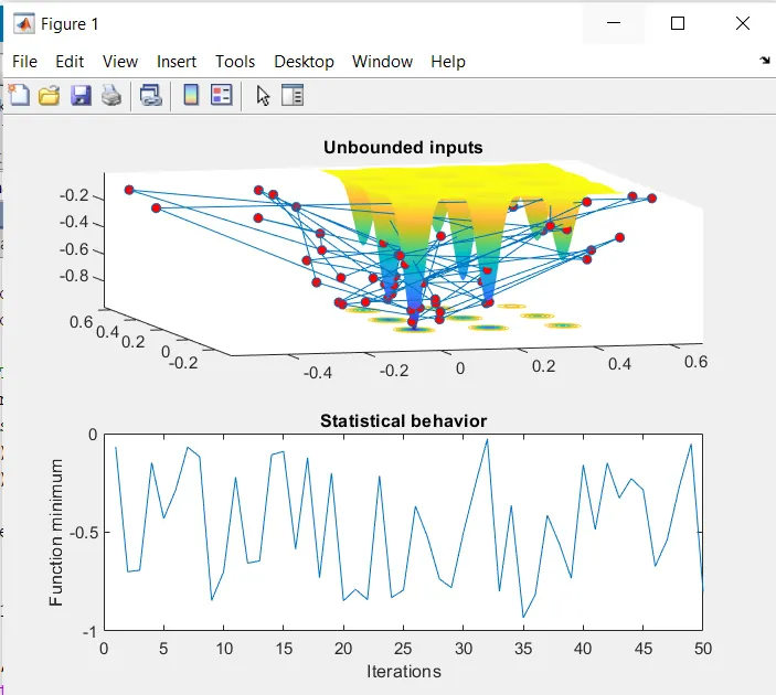
- Above figure contains two plots first one shows the stalagmite function with the optimum points but they are scattered
- The second plot shows the variation of the optimum value for 50 iterations and the values are between -1 to 0
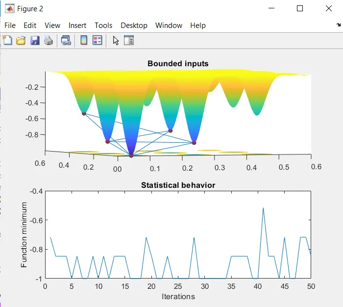
- Above figure contains two plots first one shows the stalagmite function with the optimum points converged at few peaks
- The second plot shows the variation of the optimum value for 50 iterations and the values are between -1 to -0.6 the difference is reduced as the inpurs are bounded
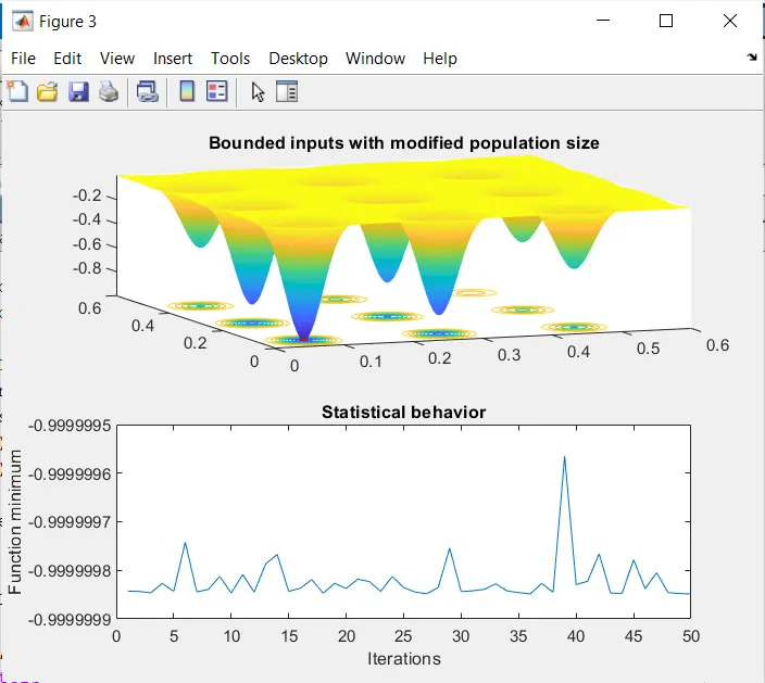
- Above figure contains two plots first one shows the stalagmite function with the optimum points converged at a single peak
- The second plot shows the variation of the optimum value for 50 iterations and the difference is reduced drastically reduced with having variation of about 0.0000001 unit and the optimum value is -0.99999965
CONCLUSIONS:
The global optimization of stalagmite function is coded and the global maxima has been determined. Concept of ga function syntax is understood and statistical behavior is also studied with three study cases where first study was a general where the inputs were unbounded, then in second study the upper and lower bounds are used to constrain the results and in the third study the population size is increased to obtain better result and all the plots were generated. The drawback of increasing the population size is it increases the run time
REFERENCES: