Week 4.1 - Genetic Algorithm
AIM:
To write the code to calculate the global maxima of the stalagmite function and explain the syntax for GA in Matlab.
OBJECTIVE:
- To write a code in Matlab to optimize the stalagmite function and find the global maxima of the function.
- To explain the concept of GA and syntax for GA in Matlab.
- To plot the graph for all 3studies and also for global maxima.
THEORY:
STALAGMITE
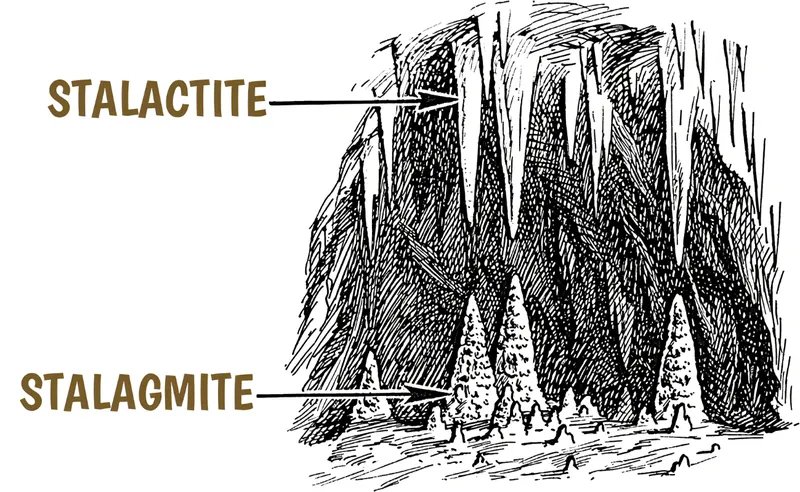
A stalagmite is a type of rock that rises from the floor of a cave due to the accumulation of materials decomposed on the floor from ceiling drippings. That is why we are using the stalagmite as the name for the program due to its shape.
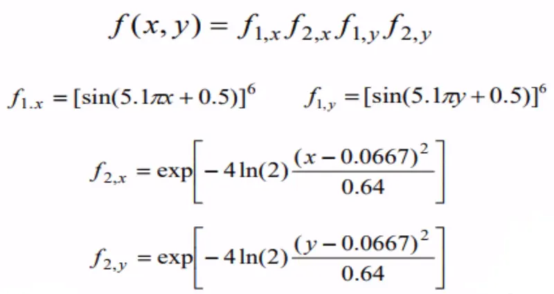
`f=-(f1x.*f2x.*f1y.*f2y)`;
`f1x=(sin(5.1*pi*x+0.5))^6`;
`f1y=(sin(5.1*pi*y+0.5))^6`;
`f2x=exp(-4*log(2)*((x-0.0667)^2/0.64))`;
`f2y=exp(-4*log(2)*((y-0.0667)^2/0.64))`;
here x and y are variables.
CODE:
Function code
function [f]=get_stalagmite(input_vector)

 x=input_vector(1);
 y=input_vector(2);

 f1x=(sin(5.1*pi*x+0.5)).^6;

  f1y=(sin(5.1*pi*y+0.5)).^6;

  f2x=exp(-4*log(2)*((x-0.0667).^2/0.64));

  f2y=exp(-4*log(2)*((y-0.0667).^2/0.64));

 f=(f1x.*f2x.*f1y.*f2y); % To find the global maxima

 f=-(f1x.*f2x.*f1y.*f2y); % To find the global minima

end
clear all
close all
clc

x=linspace(0,1,150);
y=linspace(0,1,150);

%Creating two dimensional mesh
[xx,yy]=meshgrid(x,y);

%evaluate stalagmite function
for i=1:length(xx)
    for j=1:length(yy)
        input_vector(1)=xx(i,j);
        input_vector(2)=yy(i,j);
        f(i,j)=get_stalagmite(input_vector);
    end
end

grid on
surfc(x,y,f)
hold on
shading interp
title('Unbounded inputs')
xlabel('X-axis')
ylabel('Y-axis')
output
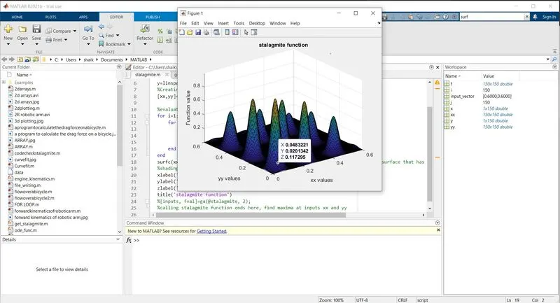
not using shading interp
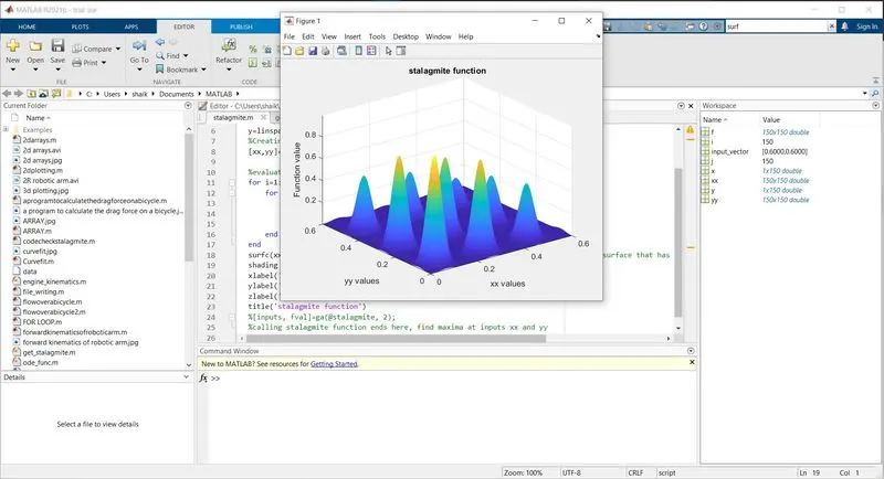
Using shading interp For global maxima
MAIN CODE:-
clear all
close all
clc

x=linspace(0,1,150);
y=linspace(0,1,150);

%Creating two dimensional mesh
[xx,yy]=meshgrid(x,y);

%evaluate stalagmite function
for i=1:length(xx)
    for j=1:length(yy)
        input_vector(1)=xx(i,j);
        input_vector(2)=yy(i,j);
        f(i,j)=get_stalagmite(input_vector);
    end
end


%% STUDY-1 Satistical behaviour of genetic algorithm
tic     %calculating the study time through tic and toc command
num_cases=50;
for k= 1:num_cases
    [input_vector, fopt(k)]=ga(@get_stalagmite,2); %calculating the optimized value of the function
    xopt(k)=input_vector(1);  %at each iteration
    yopt(k)=input_vector(2);
end
fopt=-fopt;
f=-f;
study1_time=toc;    %displaying the time taken to evaluate

%plotting the graph
figure(1)
subplot(2,1,1)

surfc(x,y,f)
hold on
shading interp
plot3(xopt,yopt,fopt,'marker','o','markersize',5,'markerfacecolor','r');
title('Unbounded inputs')
subplot(2,1,2)
plot(fopt)
xlabel('no. of Iterations')
ylabel('Function minimum')

%% STUDY-2 Satistical behaviour of genetic algorithm with upper bounds and
%lower bounds
tic     %calculating the study time through tic and toc command
num_cases=50;
for k= 1:num_cases
    [input_vector2,fopt2(k)]= ga(@get_stalagmite,2,[],[],[],[],[0;0],[1;1]); %calculating the optimized value of the function
    xopt2(k)=input_vector2(1);
    yopt2(k)=input_vector2(2);
end
fopt2=fopt2;
f=f;
study2_time=toc;    %displaying the time taken to evaluate

%plotting the graph
figure(2)
subplot(2,1,1)
surfc(x,y,f)
hold on
shading interp
plot3(xopt2,yopt2,fopt2,'marker','o','markersize',5,'markerfacecolor','r');
title('bounded inputs')
subplot(2,1,2)
plot(fopt2)
xlabel('no_of Iterations')
ylabel('Function minimum')

%% STUDY-3 Satistical behaviour of genetic algorithm by increasing no. of iterations
num_cases=50;
options = optimoptions('ga');
options = optimoptions(options,'populationsize',200);

tic     %calculating the study time through tic and toc command

for k= 1:num_cases
    [input_vector3,fopt3(k)]= ga(@get_stalagmite,2,[],[],[],[],[0;0],[1;1],[],[]); %calculating the optimized value of the function
    xopt3(k)=input_vector3(1);
    yopt3(k)=input_vector3(2);
end
fopt3=-fopt3;
f=-f;
study3_time=toc;    %displaying the time taken to evaluate

%plotting the graph
figure(3)
subplot(2,1,1)
surfc(x,y,f)
hold onh
shading interp
plot3(xopt3,yopt3,fopt3,'marker','o','markersize',5,'markerfacecolor','r');
title('bounded inputs')
subplot(2,1,2)
plot(fopt3)
xlabel('no_of Iterations')
ylabel('Function minimum')
Output:
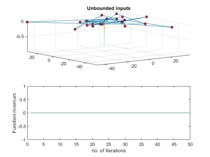
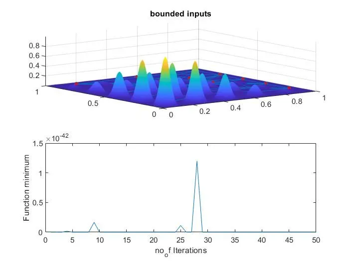
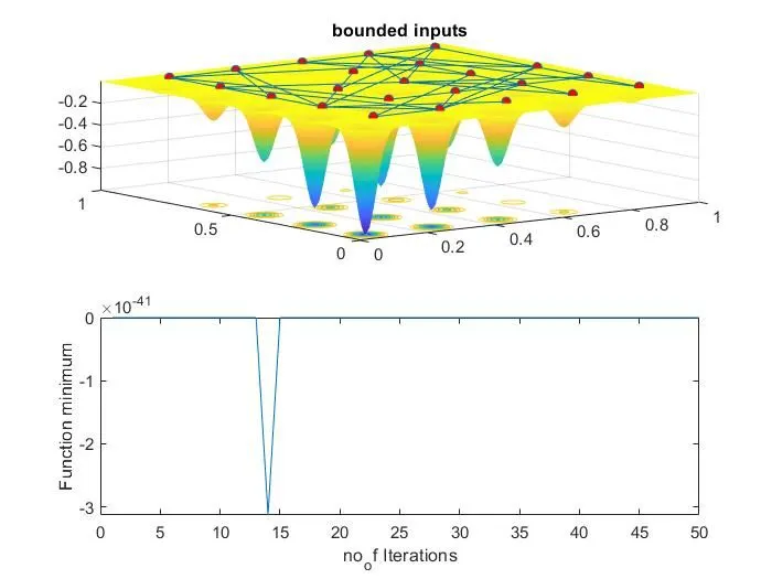
ERRORS:
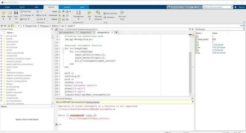
This error appears when the function code was executing a mistake.
After giving the appropriate function the error was disappear.
Explanation:
STEPWISE EXPLANATION OF THE CODE
stalagmite function for Ga
Creating a function stalagmite bypassing the input array as the argument for the variables x and y. The output of the function is stored in the variable sol.
function sol = stalagmite (input)
The first column of the input array is stored in the variable x
The first column of the input array is stored in the variable y
x=input_vector(1);
y = input_vector(2);
Stalagmite function codes
fxone = (sin(((5.1*pi).*x) +0.5)).^6;
fxtwo = exp((((x-0.0667).^2).*(-4*log(2)))./0.64);
fyone = (sin(((5.1*pi).*y)+0.5)).16;
fytwo = exp((((y-0.0667).^2).* (-4*log(2)))./0.64);
Stalagmite function values are calculated and stored in f
f = -((fxone)*(fxtwo)*(fyone)*(fytwo));
Maximization of a stalagmite Function using Genetic Algorithm//
The program starts with
clear all
close all
clc
Stores 150 values of x from 0 to 1 and,
150 values of y from 0 to 1 using linspace command.
represent cases a value of 50 is assigned to a variable n_cases.
To create a 2D array using the arrays x and y using mesh grid command.
[xx, yy) = mesh grid(x,y);
For assigning values to variables input_vector(1) and input_vector(2),
2 for loops used, Starting for loop from 1 to the length of array xx using the variable(i).
Then start one more for loop from 1 to the length of array yy using the variable (j).
Saving the value of xx as per the sequence of iteration of the for loops, in the first column of array input_vector.
Saving the value of yy as per the sequence of iteration of the for loops, in the second column of array input_vector.
Calling the function stalagmite that contains the code for evaluates the value of the function using the array input.
for i=1:length(xx)
for j=1:length(yy)
input_vector(1)=xx(i,j);
input_vector(2)=yy(i,j);
f(i,j)=get_stalagmite(input_vector);
end
end
For the study of the statistical behavior of A Genetic Algorithm, primarily a 'stopwatch' timer is started.
Starting for loop from 1 to the length of n_cases using the variable k.
Calling the genetic algorithm solver bypassing the function to solve the stalagmite function with 2 variables.
Input_vector is the array to store the optimum values if the variables of the stalagmite function as selected.
Fopt is the array to store the optimum values of the stalagmite function for all the values of x and y.
Input_vector and Fopt are the outputs of the GA.
Then saving the value of x selected by GA in the array "xopt" for every iteration of the for loop And saving the value of y selected by GA in the array "yopt" for every iteration of the for a loop.
tic
for k= 1:num_cases
[input_vector, fopt(k)]=ga(@get_stalagmite,2);
xopt(k)=input_vector(1);
yopt(k)=input_vector(2);
end
For maximizing, converting the values of the stalagmite function stored in the array "Fopt" to their negative values.
The minimum value of '- f(x)' is the maximum value of 'f(x). Then saving the time taken by the program to run the first iteration of GA in the variable Time_Study1.
fopt=-fopt;
f=-f;
study1_time=toc;
-
For plotting, the figure is generated using the figure command.
Creating a 2x1 subplot and selecting subplot 1.
(subplot(m,n,p) divides the current figure into a m*n grid and creates axes in the position specified by p)
Plotting starts with using hold on the command which retains plots in the current axes so that new plots added to the axes do not delete existing plots.
surfc command is used to create a surface plot of the values of the stalagmite function stored in the array f.
A smooth surface plot is generated by "shading interp" command.
A 3D plot is created using the plot3 command and a title is given
Subplot2 is selected.
Fopt is plotted using plot
command by using specified color and linewidth, And the axis is labeled.
figure(1)
subplot(2,1,1)
surfc(x,y,f)
hold on
shading interp
plot3(xopt,yopt,fopt,'marker','o','markersize',5,'markerfacecolor','r');
title('Unbounded inputs')
subplot(2,1,2)
plot(fopt)
xlabel('no. of Iterations')
ylabel('Function minimum')
For the study the Statistical behavior of Genetic Algorithm with Upper and Lower Bounds,
primarily a stopwatch timer is started.
Starting for loop from 1 to the length of n_cases using the variable k.
Calling the genetic algorithm solver bypassing the function to solve the stalagmite function with 2 variables.
Input_vector2 is the array to store the optimum values if the variables of the stalagmite function as selected.
Fopt2 is the array to store the optimum values of the stalagmite function for all the values of x and y.
Input_vector2 and Fopt2 are the outputs of the GA.
Then saving the value of x selected by GA in the array xopt2 for every iteration of the for loop.
And saving the value of y selected by GA in the array yopt2 for every iteration of the for loop.
tic
num_cases=50;
for k= 1:num_cases
[input_vector2,fopt2(k)]= ga(@get_stalagmite,2,[],[],[],[],[0;0],[1;1]);
xopt2(k)=input_vector2(1);
yopt2(k)=input_vector2(2);
end
For maximizing, converting the values of the stalagmite function stored in the array Fopt2 to their negative values.
The minimum value of '-f(x)' is the maximum value of 'f(x). Then saving the time taken by the program to run the first iteration of GA in the variable Time_Study2.
fopt2=-fopt2;
study2_time=toc;
For plotting, the figure is generated using the figure command.
Creating a 2x1 subplot and selecting subplot 1.
(subplot(m,n,p) divides the current figure into a m*n grid and creates axes in the position specified by p)
Plotting starts with using a hold on command which retains plots in the current axes so that new plots added to the axes do not delete existing plots.
surfc command is used to create a surface plot of the values of the stalagmite function stored in the array f.
A smooth surface plot is generated by "shading interp" command.
A 3D plot is created using the plot3 command and a title is given
Subplot2 is selected.
Fopt2 is plotted using plot command by using specified color and linewidth, And the axis is labeled.
%plotting the graph
figure(2)
subplot(2,1,1)
surfc(x,y,f)
hold on
shading interp
plot3(xopt2,yopt2,fopt2,'marker','o','markersize',5,'markerfacecolor','r');
title('bounded inputs')
subplot(2,1,2)
plot(fopt2)
xlabel('no_of Iterations')
ylabel('Function minimum')
For the study of the statistical behavior of GA by increasing the number of iterations.
Using the optimoptions function to return default options to the ga solver.
Providing the default options of the ga solver with named parameter Population Size with a value of 200.
Then a stopwatch timer is started.
Starting for loop from 1 to the length of n_cases using the variable k.
Calling the genetic algorithm solver bypassing the function to solve the stalagmite function with 2 variables.
Input_vector3 is the array to store the optimum values if the variables of the stalagmite function as selected.
Fopt3 is the array to store the optimum values of the stalagmite function for all the values of x and y.
Input_vector3 and Fopt3 are the outputs of the GA.
Then saving the value of x selected by GA in the array xopt3 for every iteration of the for loop.
And saving the value of y selected by GA in the array yopt3 for every iteration of the for loop.
num_cases=50;
options = optimoptions('ga');
options = optimoptions(options,'populationsize',200);
tic
for k= 1:num_cases
[input_vector3,fopt3(k)]= ga(@get_stalagmite,2,[],[],[],[],[0;0],[1;1],[],[]);
xopt3(k)=input_vector3(1);
yopt3(k)=input_vector3(2);
end
For maximizing, converting the values of the stalagmite function stored in the array Fopt3 to their negative values.
The minimum value of '-f(x)' is the maximum value of 'f(x). Then saving the time taken by the program to run the first iteration of GA in the variable Time_Study3.
fopt3=-fopt3;
study3_time=toc;
For plotting, the figure is generated using the figure command.
Creating a 2x1 subplot and selecting subplot 1.
(subplot(m,n,p) divides the current figure into a m*n grid and creates axes in the position specified by p)
Plotting starts with using hold on the command which retains plots in the current axes so that new plots added to the axes do not delete existing plots.
surfc command is used to create a surface plot of the values of the stalagmite function stored in the array f.
A smooth surface plot is generated by "shading interp" command.
A 3D plot is created using the plot3 command and a title is given
Subplot2 is selected.
Fopt3 is plotted using plot command by using specified color and linewidth, And the axis is labeled.
%plotting the graph
figure(3)
subplot(2,1,1)
surfc(x,y,f)
hold on
shading interp
plot3(xopt3,yopt3,fopt3,'marker','o','markersize',5,'markerfacecolor','r');
title('bounded inputs')
subplot(2,1,2)
plot(fopt3)
xlabel('no_of Iterations')
ylabel('Function minimum')
*GENETIC ALGORITHM:
A genetic algorithm makes use of techniques inspired by evolutionary biology such as selection, mutation, inheritance, and recombination to solve a problem. The most commonly employed method in genetic algorithms is to create a group of individuals randomly from a given population. The individuals thus formed are evaluated with the help of the evaluation function provided by the programmer. Individuals are then provided with a score that indirectly highlights the fitness to the given situation. The best two individuals are then used to create one or more offspring, after which random mutations are done on the offspring. Depending on the needs of the application, the procedure continues until an acceptable solution is derived or until a certain number of generations have passed.
The following steps are covered in the Genetic Algorithm.
1. Population initialization
2. fitness function calculation
3.SELECTION
3. Cross over
4. Mutation
5. Survivor selection
6. Terminate and return best
A generalized pseudo-code for a GA is explained in the following program −
GA()
   initialize population
   find fitness of population

   while (termination criteria is reached) do
      parent selection
      crossover with probability pc
      mutation with probability pm
      decode and fitness calculation
      survivor selection
      find best
   return best
The population is a subset of solutions in the current generation. It can also be defined as a set of chromosomes. There are several things to be kept in mind when dealing with the GA population −
-
The diversity of the population should be maintained otherwise it might lead to premature convergence.
-
The population size should not be kept very large as it can cause a GA to slow down, while a smaller population might not be enough for a good mating pool. Therefore, an optimal population size needs to be decided by trial and error.
The population is usually defined as a two-dimensional array of – size population, size x, chromosome size.
There are two primary methods to initialize a population in a GA. They are −
-
Random Initialization − Populate the initial population with completely random solutions.
-
Heuristic initialization − Populate the initial population using a known heuristic for the problem
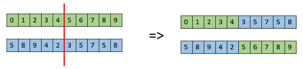
One Point Crossover
In this one-point crossover, a random crossover point is selected and the tails of its two parents are swapped to get new off-springs.
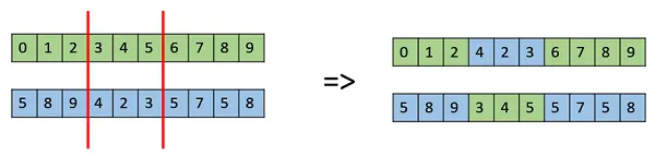
Multi Point Crossover
Multi-point crossover is a generalization of the one-point crossover wherein alternating segments are swapped to get new off-springs.
Uniform Crossover
In a uniform crossover, we don’t divide the chromosome into segments, rather we treat each gene separately. In this, we essentially flip a coin for each chromosome to decide whether or not it’ll be included in the offspring. We can also bias the coin to one parent, to have more genetic material in the child from that parent.

5. Mutation:
In simple terms, mutation may be defined as a small random tweak in the chromosome, to get a new solution. It is used to maintain and introduce diversity in the genetic population and is usually applied with a low probability – pm. If the probability is very high, the GA gets reduced to a random search.
The mutation is the part of the GA which is related to the “exploration” of the search space. It has been observed that mutation is essential to the convergence of the GA while the crossover is not.
6. Termination:
The termination condition of a Genetic Algorithm is important in determining when a GA run will end. It has been observed that initially, the GA progresses very fast with better solutions coming in every few iterations, but this tends to saturate in the later stages where the improvements are very small. We usually want a termination condition such that our solution is close to the optimal, at the end of the run.
SYNtax for GA:
x = ga(@func,nVars)
x = ga(@func,nVars,A,b)
x = ga(@func,nVars,A,b,Aeq,beq)
x = ga(@func,nVars,A,b,Aeq,beq,lb,ub)
x = ga(@func,nVars,A,b,Aeq,beq,lb,ub,nonlcon)
x = ga(@func,nVars,A,b,Aeq,beq,lb,ub,nonlcon,options)
[x,fval] = ga(...)
Inputs