Week 3 - Solving second order ODEs

AIM:- To create a simple pendulum oscillation and create a movie using Matlab software by solving the second-order ODE

SIMPLE PENDULUM:- A simple pendulum consists of a mass 'm' hanging from a string of length 'L' and fixed at a pivot point 'P'.When displaced to an initial angle and released, the pendulum will swing back and forth with the periodic motion.

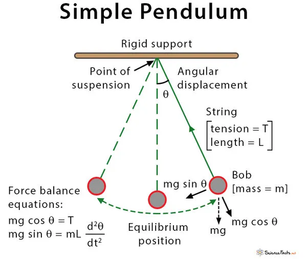
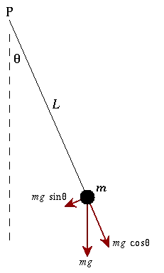
The period for a simple pendulum does not depend on the mass or the initial angular displacement, but depends only on the length L of the string and the value of the gravitational field strength g,

`T=2pi sqrt(l/g)`

applying newtons second law of motion to a simple pendulum we can get the equation of motion for a pendulum with a damping coefficient that

`(d^2theta)/(dt^2)+b/m ((d theta)/dt)+g/l(sintheta)=0`

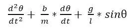
in the above equation

B= damping coefficient

m= mass of the BOB in 'KG'

L= length of the pendulum in 'm'

g= acc.due to gravity

now we solve higher ode we can break the equation into first-order ODE

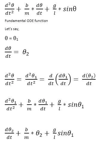
`((dθ2)/dt)=−(b/m)(θ2)−(g/l)(sinθ1)`

`d/dt((theta1) /(theta2))=[(theta2) / (−(b/m)(θ2)−(g/l)(sinθ1) ]`

the above equation is solution vector in the form of matrix

INPUTS:-

The input parameters are given below

l=1 in 'm'

b=0.05

m=1 in 'kg'

g=9.81

angular displacement=0;

angular velocity=3;

time span=[0,20];

STEPS:- explain the the code in step wise

1) entering the input parameters

2) set the angular displacement and angular velocity are given in the form of the array into a new variable is known by "y_0" and then the time period for the oscillation is given with the help of linspace command from 0 to 20 with 800 points and that variable is known by "t_span"

3) solving ODE equation with the help of ODE command in MATLAB

[t,amplitude]=ode45(@(t,theta)ode_func(t,theta,b,g,l,m),t_span,y_0)

In this we are defining the ODE45 is the function of t and theta is only dependent and independent variables, then we added the time span and initial conditions on this command

4) plotting graph which shows the angular displacement and angular velocity with respect to time and we can observe the changes in the graph by changing the damping coefficient

5)using for loop command to create animation here we get the value with the range operator to the length of the amplitude value1, which is angular displacement values. after that, we are assigning the new variable called (i)

next giving the coordinates of string and bob (x0,y0) and (x1,y1)

6) plotting figure in for loop command where is fixed support and string with bob

7) finally creating a video file with the help of get frame, and movie command

Main Code:-

clear 
close all
clc

b=0.05;  % damping co efficient
g=9.81;  % acc.due to gravity
l=1;     % length of the pendulum in M 
m=1;   % mass in KG

%initial condition
y_0=[0 3];  % angular displacement=0 & angular velocity=3 

%time points
t_span=linspace(0,20,100);

%solve ode
[t,amplitude]=ode45(@(t,theta)ode_func(t,theta,b,g,l,m),t_span,y_0);

figure(1)
plot(t,amplitude(:,1))
hold on
plot(t,amplitude(:,2))
xlabel('time')
ylabel('amplitude')
legend('angulaar displacement','angular velocity')

% animation
ct=1;
for i=1:length(amplitude(:,1))
    x0=0;
    y0=0;

    x1=1*sin(amplitude(i,1));
    y1=-1*cos(amplitude(i,1));

    figure(2)
    plot([-1.5 1.5],[0 0],'LineWidth',3,'Color','g')
    hold on
    plot([x0 x1],[y0 y1],'LineWidth',1,'color','m')
    plot(x1,y1,'marker','o','markerFace','b','markersize',10)
    hold off
    axis([-2,2 ,-2,2])
    pause(0.03)

    M(ct)=getframe(gcf);  % capture the current figure using getframe command
    ct=ct+1;
end

movie(M)
videofile=VideoWriter('simple_pendulum oscillation.avi');
open(videofile)
writeVideo(videofile,M)
close(videofile)

Function code :

using function is the set of commands used to perform the task. The main purpose of this we can run this with any set of values when needed. This will reduce the main program size. In Matlab, the function name & the function file should be stored in the same name as well as in the same path.

function [dtheta_dt]=ode_func(t,thetaa,b,g,l,m)

         theta1=thetaa(1);
         theta2=thetaa(2);
         dtheta1_dt=theta2;
         dtheta2_dt=(-b/m)*theta2-(g/l)*sin(theta1);
         dtheta_dt=[dtheta1_dt;dtheta2_dt];
         
end

In the above command ode_func is the function name with the set of input values that will be declared in the main program. Then we are storing the output with a new variable name called [dtheta_dt].

Plotting graph:

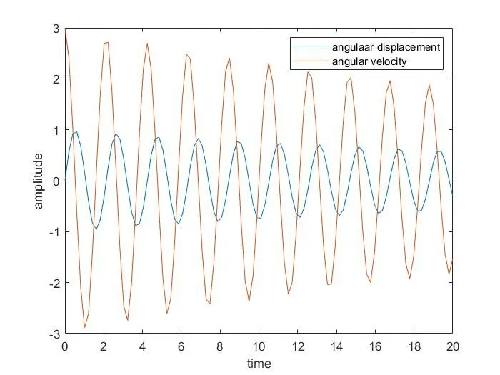
In the below plot the damping co-efficient was changed as b=0.5; so the period of oscillation that is the angular displacement of the pendulum is reduced as well as the angular velocity

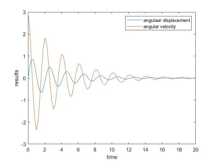
From the above experiment, we can say that with the assumption of small angles, frequency and period of the pendulum are independent of the initial angular displacement amplitude

Errors:-

when i use the marker command

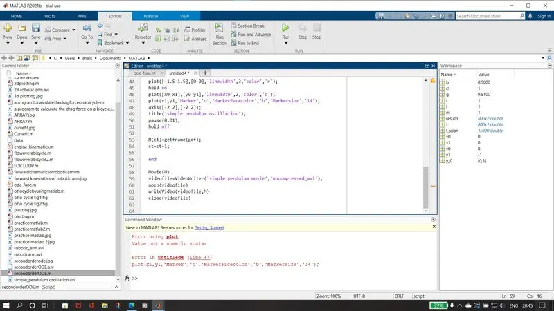
taken the help from the search bar in Matlab and use it.

Here the movie link below

https://drive.google.com/file/d/1akKLAzq8He7HcQXblrHlid6oyg3MH47Q/view?usp=sharing

https://www.youtube.com/watch?v=fsvniGjKdkQ