Week 4.1 - Genetic Algorithm

AIM :

To write a code in MATLAB to optimize the stalgamite function and to find the global maxima of the function.

THEORY :

Generic Algorithm (GA) is a search based optimization techniques based on the principles of Genetics and Natural selection. It is fequently used to find optimal or near optimal solutions which diffiult problems otherwise it would take lifetime to solve.

Optimization is a process of making something better.In any process we have a set of inputs and set of outputs as shown in the figure.

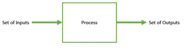
Optimization refers to finding the values of inputs in such a way we get the "best" output values. The definition of best varies from problem to problem , but in mathematical terms it refers to maximizing and minimizing one or more objective functions, by varying the input parameters.

Generic Algorithms are sufficiently randomized in nature, but they perform much better than random local search. The generic algorithms uses three main types of rules at each step to create the next generation from the current population.

• Selection rulesselect the individuals, called parents, that contribute to the population at the next generation.
• Crossover rules combine two parents to form children for the next generation.
• Mutation rulesapply random charges to individual parents to form children.

How the Generic Algorithm works ?

The following outline summarizes how the generic algorithm works:

• The algorithm begins by creating a random initial population.
• The algorithm then creates a sequence of new populations. At each step, the algorithm uses the individuals in the current generation creates the next population.
• To create the new population , the algorithm performs the following step:
• Scores each member of the current population by computing its fitness value. These values are called as the raw fitness scores.
• Scaling the raw fitness scores to convert them into a more usable range of values.These scaled values are called the expectation values.
• Selects members called parents, based on their expectation.
• Some of the individuals in the current populalation that have lower fitness are chosen as elite. These elite individuals are passed to the next population.
• Produces children from the parents.Children are produced either by making random changes to a single parent -mutation-or by combining the vector entries of a pair of parents.
• Replaces the current population with the children to form the next generation.

Operators of Generic Algorithm :

Once the initial generation is created, the algorithm evolve the generation using following operators :

1. Selection Operator : The idea is to give preferences to the individuals with good fitness scores and allow them to pass genes to the successive generations.
2. Roulette Wheel Selection :
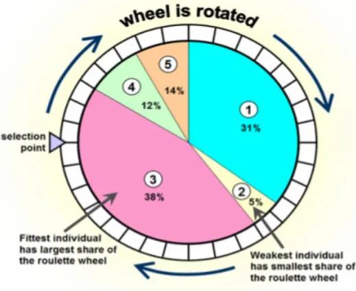
3. In a roulette wheel selection, the circular wheel is divided with respect to the filter individual. A fixed point is chosen on the wheel circumference as shown and the wheel is rotated. The region of the wheel which comes in front of the fixed point is chosen as the parent. For the second parent , the same process is repeated.
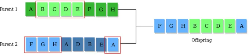
4. Crossover operator : This represents mating between individuals. Two individuals are selected using selection operator and crossover sites are chosen randomly. Then the genes at the these crossover sites are exchanged thus creating a completely new individual(offspring).
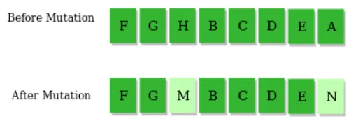
5. Mutation operator : The key idea is to maintain the diversity from one generation of population of chromosomes to the next. If mutation is not performed , the chromosomes will become to similar to each other, convergebce takes place soon and results in local minima.Example- Insert random genes in offspring , here random genes are inserted to maintain the diversity.

STEP-WISE EXPLANATION :

• Program starts with clear all, close all, clc., which is used to clear all the stored datas in workspace, command window
• Defining the search space using the linspace command that will provide 150 values between 0 and 0.6.
• Next "Meshgrid" command to be used to create a 2 dimentional array based on our one dimentional array values.
• Evaluating the Stalgamite function for each value of X and Y.
• The function code has been given below the main program.
• To calculate the maxima, a new function code has been written by using the below formula,

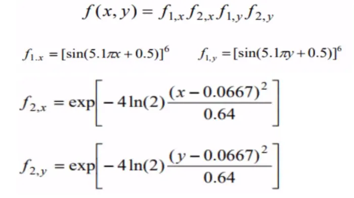
• Generally, Generic algorithm is used to calculate the minimum value only , but here our task is to find out the global maxima of the function.
• so, to get the global maxima of the function,we can use the below formula,

`f(x,y) = -(f_1,_x * f_2,_x * f_1,_y * f_2,_y)`

MATLAB PROGRAM :

From this code we can able to find out the global maxima of the function.

clear all
close all
clc

% Initializing
x = linspace(0,0.6,150);
y = linspace(0,0.6,150);
num_cases =50; % number of iterations to be performed

% creating a 2Dimentional mesh
[xx yy] = meshgrid(x,y);

% Evaluating the stalagmite function
for i = 1:length(xx) 
    for j = 1:length(yy)
        input_vector(1)= xx(i,j); % just assigning the x and y values in input vector variables
        input_vector(2)=yy(i,j);
        f(i,j)=stalagmite1(input_vector); % calling the function stalagmite1
        
    end
end
% study 1 -statistical behaviour for unbounded condition
% Using tic - toc command for calling the iterations
tic   
for i = 1:num_cases 
    [inputs1 ,fopt(i)] = ga(@stalagmite1,2);
    xopt1(i) = inputs1(1);
    yopt1(i) = inputs1(2);
end

study1_time = toc

% plotting using subplot command where two different plots can be shown in a single figure
figure(1)
subplot(2,1,1)
hold on
surfc(x,y,-f)
shading interp
plot3(xopt1,yopt1,-fopt,'marker','o','MarkerSize',5,'MarkerFaceColor','r') % plot3 command used to plot x,y & z axis 
title('unbounded inputs')
subplot(2,1,2)
plot(-fopt)
xlabel('Iterations')
ylabel('Function maximum')


% Study 2 -Statistical behaviour with uppper and lower bounds

tic
for i = 1: num_cases
     [inputs2 ,fopt(i)] = ga(@stalagmite1,2,[],[],[],[],[0,0],[1,1]);
     xopt2(i) = inputs2(1);
     yopt2(i) = inputs2(2);
end

study2_time = toc

% plotting
figure(2)
subplot(2,1,1)
hold on
surfc(x,y,-f)
shading interp
plot3(xopt2,yopt2,-fopt,'marker','o','MarkerSize',5,'MarkerFaceColor','r')
title('Bounded inputs');
subplot(2,1,2)
plot(-fopt)
xlabel('Iterations')
ylabel('Function maximum')

% Study 3 -increasing GA iterations
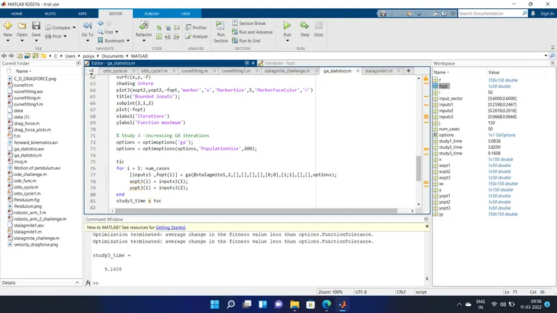
options = optimoptions('ga');
options = optimoptions(options,'PopulationSize',200); % Setting population size as 200 so that function maxima can be found out easily

tic
for i = 1: num_cases
     [inputs3 ,fopt(i)] = ga(@stalagmite1,2,[],[],[],[],[0;0],[1;1],[],[],options);
     xopt3(i) = inputs3(1);
     yopt3(i) = inputs3(2);
end 
study3_time = toc
 
% plotting 
figure(3)
subplot(2,1,1)
hold on
surfc(x,y,-f)
shading interp
plot3(xopt3,yopt3,-fopt,'marker','o','MarkerSize',5,'MarkerFaceColor','r')
title('Bounded inputs with modified population size');
subplot(2,1,2)
plot(-fopt)
xlabel('Iterations')
ylabel('Function maximum')

STALGAMITE FUNCTION CODE :

• 'stalagmite1' is the name of the function that i gave for this program.
• This function calculates the formulas which i mentioned in the above steps.

% Function code generation

function [result] = stalagmite1(input_vector)
x = input_vector(1);
y = input_vector(2);

fx1 = (sin(5.1*pi*x + 0.5)).^6;
fy1 = (sin(5.1*pi*y + 0.5)).^6;
fx2 = exp((-4*log(2)*((x-0.0667).^2)/0.64));
fy2 = exp((-4*log(2)*((y-0.0667).^2)/0.64));

result =-(fx1*fy1*fx2*fy2); 

end

STUDY 1 : Statistical behaviour for unbounded condition

• FOR LOOP is used to run the code for 50 iterations ,because ga doesn't know the actual space.
• tic-toc command is used for calling the iterations and also used to store the time period of evaluation.
• A new function is created @stalagamite that will pass 2 variable as inputs and stores the output in fopt(i).
• Later i have stored the values of x and y in 'xopt' and 'yopt'.
• Next is plotting using 'subplot' command where 2 plots can be shown in a single figure.
• To see the output 'surfc' command is used and also 'shading interp' command used to get the smooth plots without grid lines.
• Output graphs has been shown below,

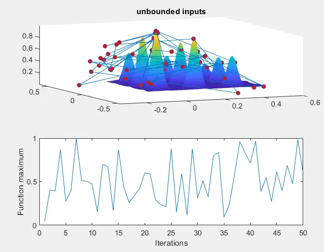
• From the above diagram, we can see that the global maxima value may come from outside the search space also.
• so, the exact maximum value cannot be found from this.
• Studytime for this process is about 3.08 secs.

STUDY 2: Statistical behaviour with bounded and unbounded inputs :

• In this study, we are assigning the boundary values for search space.
• Upper and lower bounds are given in ga syntax as between 0 and 1.
• Previously we have the plots of unbounded condition, values were not clear so, now syntax is applied with bounded values.
• The syntax used here is, [inputs ,fopt(i)] = ga(@stalagmite1,2,[],[],[],[],[0,0],[1,1])
• 0 and 1 are the upper limit and the lower limit.
• The output is shown below,

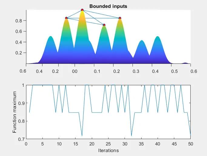
• Here from the graph it seems that the function maximum value is between 4 points.
• It is better assumption when compared with the previous study.
• Because of using upper and lower bounded values , the global maxima of the function is well predicted.
• Even though much better than the previous case, this is not the exact result what we required.
• Studytime for this process is about 3.82 secs, bit similar to the first case.

STUDY 3: Increasing GA iterations :

• From the 2 cases, we cannot find the exact maximum value so, i have increased the GA iterations.
• With less population size, it's difficult to find the global maxima.
• So, increasing the population size to 200 and applying the constaraints 'optimoptions' and saving the values in 'options' .
• Output of this study is given below,

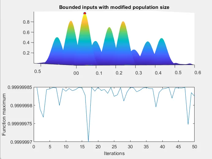
• So, the global maxima of the function is predicted between 0.9999999 to 1 .
• By increasing the number of iterations and apllying the constraints , we can acheive this.
• Studytime for this process is about 9.16 secs ,bit it takes little more timeperiod to evaluate.

OUTPUT :

SYNTAX FOR GA :

Syntax for ga = ga(@stalagmite,2,[],[],[],[],[0;0],[1;1],[],[],options)

ga(fun,nvars,A,b,Aeq,beq,lb,ub,nonlcon,options)

• ga- To find the minimum of function using generic algorithm
• fun- finds a local minimum to function
• nvars- number of variables
• A- Linear inequality constraints, specified as a real matrix
• b- Linear inequality constraints, specified as a real vector
• Aeq- Linear inequality constraints, specified as a real matrix
• beq - Linear inequality constraints, specified as a real matrix
• lb- lower bound
• ub- upper bound
• nonlcon- Non linear constraints
• options- Optimization process

SIGNIFICANCE OF RUNNING MULTIPLE ITERATIONS :

• Without running multiple iterations ,finding the global maxima is difficult.
• The number of iterations helps us to evaluate the process easily.

CONCLUSION :

• The concept of Generic Algorithm, finding global maxima of the function, syntax of the GA has been explained clearly.