Week 3 - Solving second order ODEs

AIM:

The main objective of the project is to simulate the motion of a simple pendulum using MATLAB by solving a second order ODE.

FORMULA:

• The second order ODE equation of the pendulum with damping is given as

`d^2 theta/dt^2 + (b/m)(d theta/dt)+(g/l)sin theta = 0` ________(1)

• The above equation can be solved once we break down into two First-order ODE equations.

Let assume, `theta = theta1`

`d theta/dt = d theta1/dt = theta2`_________(2)____ First ODE

`d^2theta/dt^2 = d/dt(d theta/dt) = d/dt(theta2)`________(3)

Substitute `theta = theta1` in equation (1)

`d^2 theta1/dt^2 +(b/m)(d theta1/dt) + (g/l)sin theta1 = 0`_________(4)

Apply (2) & (3) in (4)

`d theta2/dt + (b/m)theta2 + (g/l)sin theta1 = 0`

`d theta2/dt = (-b/m)theta2-(g/l)sin theta1`________ Second ODE

`d/dt[(theta1),( theta2)] = [ (theta2),((-b/m)*theta2 - (g/l)*sin theta1)]`

• lets assume ,

`[(theta1),(theta2)] = theta`

• The given values are

g = 9.81 - gravity in `m/s^2`

L = 1 metre - length of the pendulum

m = 1 kg - mass of the ball

b = 0.05 - damping coefficient

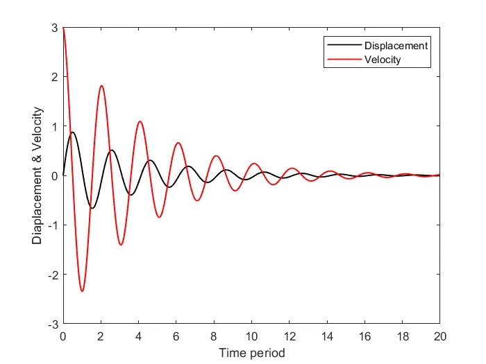
t_span = 0-20 secs - Time period

Angular displacement = 0

Angular Velocity = 3 rad/sec

MATLAB Program:

% 2nd order ODE equations for simple pendulam

% BAsic commands

clear all
close all
clc

b = 0.05; % damping co-efficient
g = 9.81; % gravity in m/s^2
m = 0.1;  % mass of the ball in kg
l = 1;    % length of the pendulum in m
 
% Initial conditions for displacement and velocity

theta_0 = [0;3]; % 0- initial displacement of the pendulum 
                 % 5- initial velocity value

% Initializing the time array how far the integration need to be done

t_span = linspace(0,20,500); % t_span is time array & it will give 500 values between 0 to 10 secs

% Solving ODE equations

[t,results] = ode45(@(t,theta)ode_func(t,theta,b,g,l,m),t_span,theta_0);

% plotting
plot(t,results(:,1),'LineWidth',1,'Color','k')
hold on
plot(t,results(:,2),'LineWidth',1,'Color','r')
xlabel('Time period')
ylabel('Diaplacement & Velocity')
legend('Displacement','Velocity')

Function code generation:

ode_func is the name of this program, and the output of this program can be used at any time in some other program.

function [dtheta_dt] = ode_func(t,theta,b,g,l,m)    % generating function
      theta1 = theta(1)
      theta2 = theta(2)
      dtheta1_dt = theta2;                          % First ODE equation
      dtheta2_dt = -(b/m)*theta2-(g/l)*sin(theta1); % second ODE equation
      dtheta_dt = [dtheta1_dt;dtheta2_dt ]          % mentioned as column matrix
end

Output graph:

Program to simulate the motion of the pendulum:

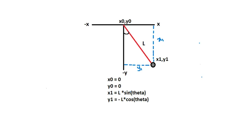
• Lets assume,

% program for the motion of the pendulum

x0 = 0; % X,Y coordinates assumed as 0
y0 = 0;
ct = 1; % A variable to do counter up process

% FOR loop to repeat the process until the given time period completes

for i = 1:length(t) 
    theta = results(i,1);
    x1 = l*sin(theta); % x1 & y1 coordinates can be found out using this formula
    y1 = -l*cos(theta);
   
   % plotting 
   plot([-1 1],[0 0],'LineWidth',5,'Color','k'); % plotting the fixed end of the pendulum
   hold on   
   plot([x0 x1],[y0 y1],'b'); % Represents the  position of the pendulum
   hold on

   % Marker
   plot(x1,y1,'Marker','o','MarkerSize',15,'MarkerFaceColor','g') % plotting the boll and its color,size,shape
   hold off
   axis([-5 5 -5 0]) % Assigning the values for xaxis, yaxis
   grid on
   M(ct) = getframe(gcf); %get current frame command collects all the frames 
   ct = ct + 1; % incrementing the count

end
% Program for animation video
movie(M) % where M is an array to get all the figures while executing
videofile = VideoWriter('Motion of pendulum.avi','Uncompressed AVI'); %Videofile is the variable to save the movie
open(videofile)
writeVideo(videofile,M) % Writing the videofile, which contains all the figures
close

Output :

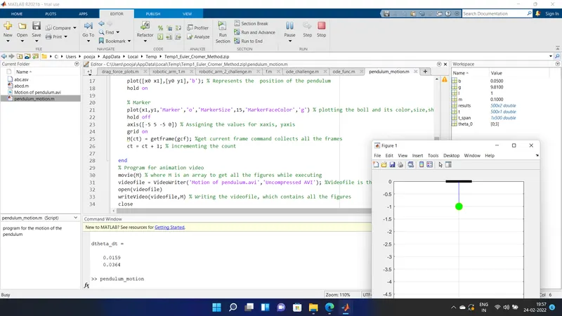
Animation video link is given below:

https://youtu.be/MYiS5EgFHII

Error Faced while programming:

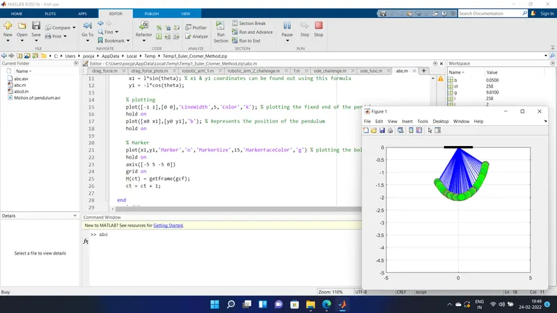
It tooks a lot of time to realize that i made a mistake on line 22. I should give hold off command. Because of using hold on command, all the frames have been showing in the animation.

Conclusion:

From this programming we can able to see the motion of the pendulum for the given period of time.