Project 1 - Parsing NASA thermodynamic data

AIM :

• The aim is to write a function that extracts the 14 co-efficients and calculate the Enthalpy, Entropy and Specific heats for all the species in the given NASA THERMODYNAMICS datafile.
• To calculate the molecular weight of each species.
• To plot the Cp, Enthalpy, Entropy for the local temperature range.
• To save the plots as images with appropriate names and dump them in seperate folders for each species with suitable name and also it need to generate automatically.

STEPWISE EXPLANATION :

• Starting the program with clear all , close all, clc used to remove the previous items from the workspace, close one or more figures and clears the command window.
• 'fopen' command is used to read data from the given datafile(THERMO.DAT)
• To get a line from any text file 'fgetl(File ID)' command is used.
• First line is the heading of the file , I am using the variable called 'header' to read the line from the given data file.
• Next line is about three global temperatures and to read the data from the text file 'fscanf' command is used.
• Next three lines are the comments and to skip those lines 'for loop' is used.
• For loop can be used here , because i have to findout 53 species from the fiven datafile , so im repeating the below process for 53 iterations like, i = 1:53.
• Local temperatures and the species name can be find out from the next line.
• To find the co-efficients 'strfind' command is used to find the sting in that particular line .

A = strfind(co_effs,'E')
a1 = co_effs(1:A+3) -------> First co-efft

• 'E' is the common letter in all the co-efficients, so it's easier to find all co-efficients.
• a2 can be be found out by a2= co_effs(A(1)+4:A(2)+3)------> second co-efft
• 'str2double' command coverts the string into real or complex numeric values.
• a1 to a5 - 5 co-efficients can be found out and get the next line and find the next set of co-efficients and repeat the same.
• a1 to a14 -all the 14 co-efficients can be found out upoto this process.
• Initializing R= 8.314 , where R = universal gas constant
• Cp, H, S are the Specific heat, Enthalpy, Entropy.
• The below formula has to be used to calculate Cp,H,S

• T is the temperature and linspace command is used to generate 1000 values between the local low temperature and local high temperature.
• In this challenge it is given that first 7 co-efficients are high temperature co-efficients and second 7 co-efficients are low temeprature co-efficients and the temperatures must be local temperatures only.
• Using if and else loop if T is less than the local mid temperature then a8 to a14 will be used and vice versa.
• Cp , H and S are calculated for 1000 values and so plotting can be done in three different figures.

MATLAB PROGRAM :

% Parsing NASA thermodynamic data

clear all % Removes items from the Workspace
close all % Close one or more figures
clc       % Clear Command Window

% Initializing the inputs
f1 = fopen('THERMO.dat','r');  % Reading data from the data file
header = fgetl(f1);             % Reading line from the file
temperature = fscanf(f1,'%f'); % Reading data from the text file
global_low_temp = temperature(1);
global_mid_temp = temperature(2);
global_high_temp = temperature(3);

% skipping the comments (Next three lines)
comments = 1:3;
for i =1: length(comments)
    skip_comments = fgetl(f1);
end

% For loop to calculate the 53 species 
for j = 1:53

   Next_line = fgetl(f1);
   cell = strsplit(Next_line,' '); % strsplit used to split the strings in a line
   end_line = length(cell);
   species_name = (cell{1});
   
   % Finding local temperatures
   local_low_temp =  str2double(cell{end_line-3});
   local_high_temp = str2double(cell{end_line-2});
   local_mid_temp=  str2double(cell{end_line-1});

   % Calculating the co-efficients of the first line
   co_effs = fgetl(f1);
   A = strfind(co_effs,'E'); % Finding the particular string from a line
   a1 = co_effs(1:A+3);
   a1 = str2double(a1); % converts string into numeric values
   a2= co_effs(A(1)+4:A(2)+3);
   a2 = str2double(a2);
   a3= co_effs(A(2)+4:A(3)+3);
   a3 = str2double(a3);
   a4= co_effs(A(3)+4:A(4)+3);
   a4 = str2double(a4);
   a5= co_effs(A(4)+4:A(5)+3);
   a5 = str2double(a5);
   % Calculating the co-efficients of the second line
   fgetl(f1);
   B = strfind(co_effs,'E');
   a6 = co_effs(1:B+3);
   a6 = str2double(a6);
   a7= co_effs(B(1)+4:B(2)+3);
   a7 = str2double(a7);
   a8= co_effs(B(2)+4:B(3)+3);
   a8 = str2double(a8);
   a9= co_effs(B(3)+4:B(4)+3);
   a9 = str2double(a9);
   a10= co_effs(B(4)+4:B(5)+3);
   a10 = str2double(a10);
   % Calculating the co-efficients of the third line
   fgetl(f1);
   C = strfind(co_effs,'E');
   a11 = co_effs(1:C+3);
   a11 = str2double(a11);
   a12= co_effs(C(1)+4:C(2)+3);
   a12 = str2double(a12);
   a13= co_effs(C(2)+4:C(3)+3);
   a13 = str2double(a13);
   a14= co_effs(C(3)+4:C(4)+3);
   a14 = str2double(a14);

   % R is the universal gas constant
   % Cp is the Specific heat
   % H is the Enthalpy
   % S is the Entropy

    R = 8.314; 
    T = linspace(local_low_temp,local_high_temp,1000); % linspace generates 1000 values between local low temp and local high temp

    if T<local_mid_temp
       Cp = (a8 + a9*T + a10*T.^2 +a11*T.^3 +a12*T.^4)*R; 
       H = (a8 +a9*T/2 +a10*T.^2/3 + a11 *T.^3/4 +a12*T.^4/5 +a13./T)*R.*T;
       S = (a8*log(T) + a9*T + a10*T.^2/2 + a11*T.^3/3 + a12*T.^4/4 + a14)*R; 
    else
       Cp = (a1 + a2*T + a3*T.^2 +a4*T.^3 +a5*T.^4)*R; 
       H = (a1 +a2*T/2 +a3*T.^2/3 + a4 *T.^3/4 + a5*T.^4/5 +a6./T)*R.*T;
       S = (a1*log(T) + a2*T + a3*T.^2/2 + a4*T.^3/3 + a5*T.^4/4 + a7)*R; 
    end

% plotting 

figure(1) 
plot(T,Cp,'linewidth',3,'Color','K')
grid on
xlabel('Temperature')
ylabel('Specific Heat Cp')
title(sprintf('%s',species_name))

figure(2)
plot(T,H,'linewidth',3,'Color','g')
grid on
title(sprintf('%s',species_name))
xlabel('Temperature')
ylabel('Enthalpy')

figure(3)
plot(T,S,'linewidth',3,'Color','b')
grid on
xlabel('Temperature')
title(sprintf('%s',species_name))
ylabel('Entropy')

cd('C:\POOJASRI')
mkdir(species_name) % making new folder name
cd(species_name)    % change curent folder
saveas(1,'Temperature vs Specific heat','jpg') % save figure to jpg file format
saveas(2,'Temperature vs Enthalpy','jpg')
saveas(3,'Temperature vs Entropy','jpg')
cd ..    % level up from the current folder

% CALCULATING MOLECULAR WEIGHT OF THE SPECIES 

mol_weight = 0; % Initializing 
elements = ['O','C','H','Ar','N']; % These are the main species in the datafile
atomic_wght = [15.999 12.010 1.007 39.948 14.006]; % Atomic weight of the corresponding above elements 

 for ii = 1:length(species_name)
    for jj = 1: length(atomic_wght)
        if strcmp(species_name(ii),elements(jj)) % Comparing the strings
            mol_weight = mol_weight + atomic_wght(jj);
            position = jj;
        end 
    end
    n = str2double(species_name(ii));
    if n>1
        mol_weight = mol_weight+ atomic_wght(position)*(n-1); 
    end
  end
fprintf('Molecular weight of %s = %f\n\n',species_name,mol_weight) % printing the molecular weight of the species

end

SAVING PLOTS AS IMAGES AUTOMATICALLY :

• 'mkdir(Folder_name)' command is used for making new folder.
• 'cd(folder_name)' command used to change into current folder.
• 'saveas(fig,filename)' - this syntax is used to save figure into specific file format.
• All the 3 figures with appropriate file format has been given.
• This process will save the plota as images in desktop, and if we need to change the address we can simply use 'cd(address path)'.

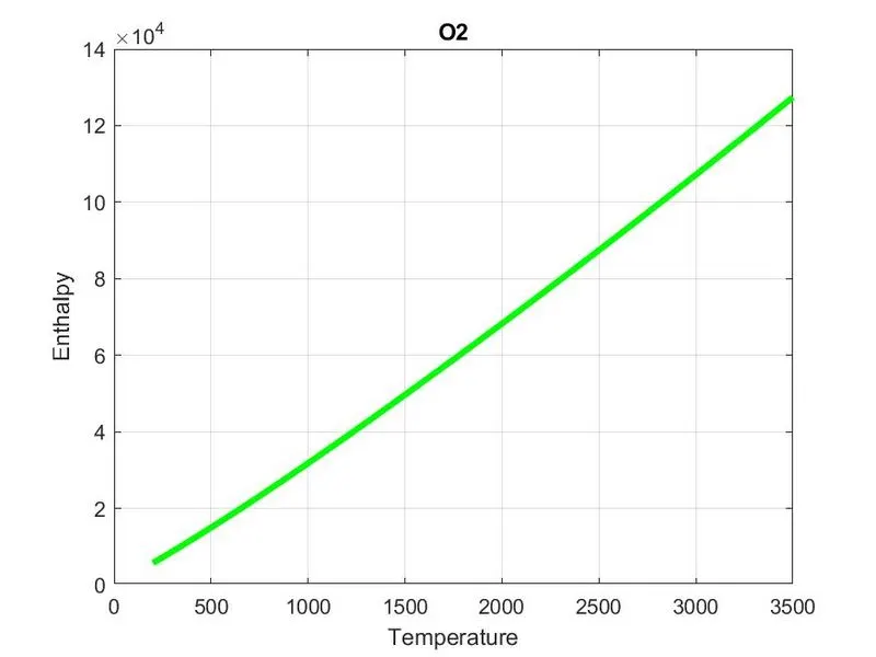
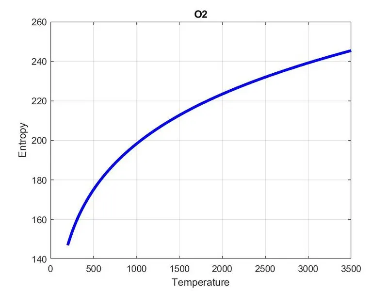
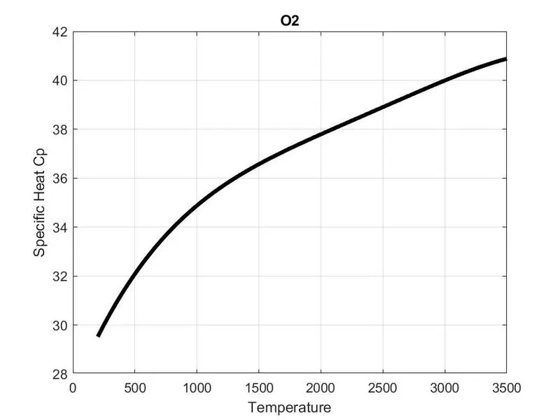
PLOTS FOR O2:

• Temperature Vs Enthalpy :

• Temperature Vs Entropy :

• Temperature Vs Specific heat :

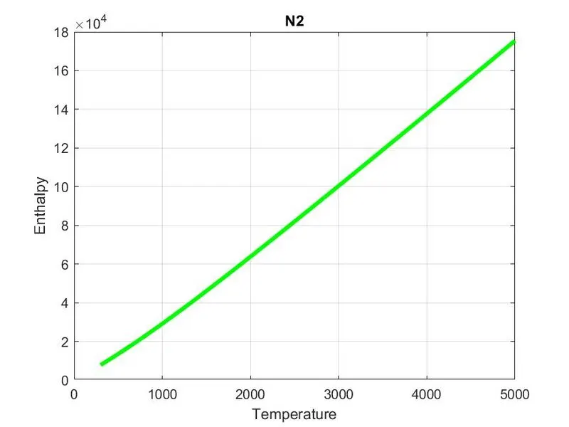
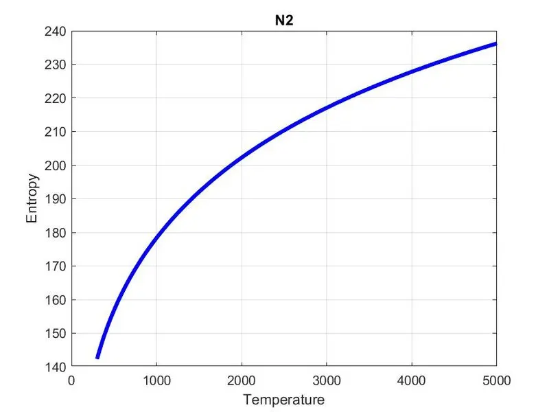
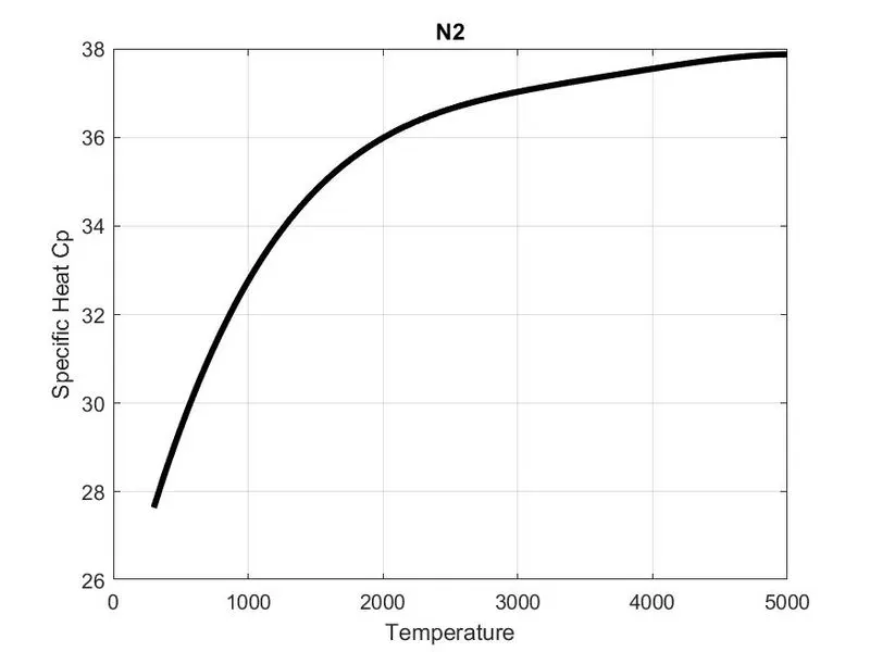
PLOTS FOR N2 :

• Temperature Vs Enthalpy :

• Temperature Vs Entropy :

• Temperature Vs Specific heat :

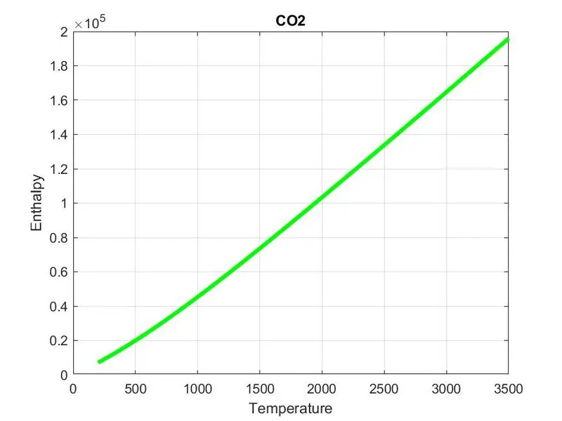
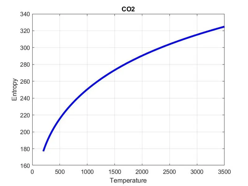
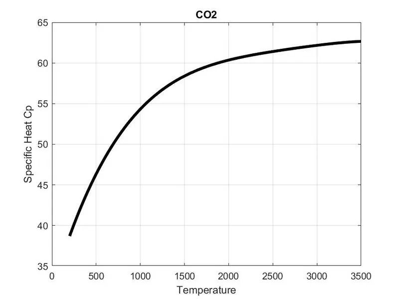
PLOTS FOR CO2 :

• Temperature Vs Enthalpy :

• Temperature Vs Entropy :

• Temperature Vs Specific heat :

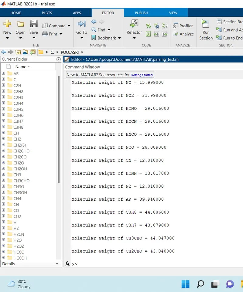
CALCULATING MOLECULAR WEIGHT OF THE SPECIES :

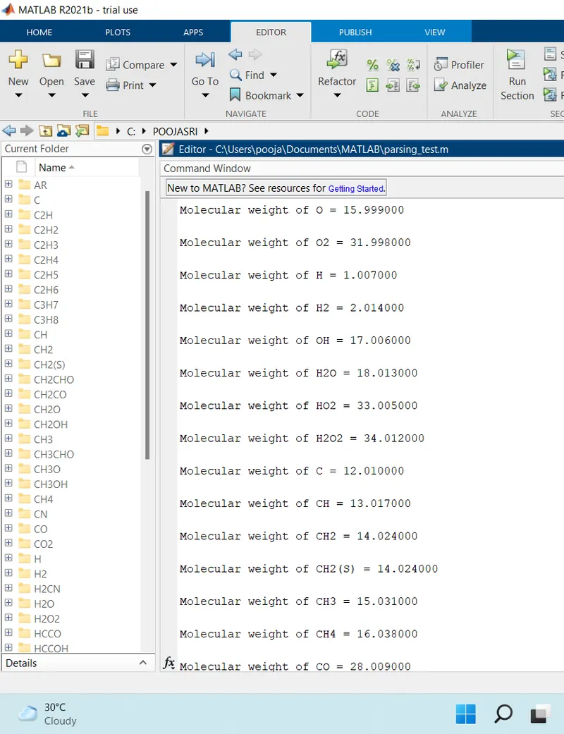
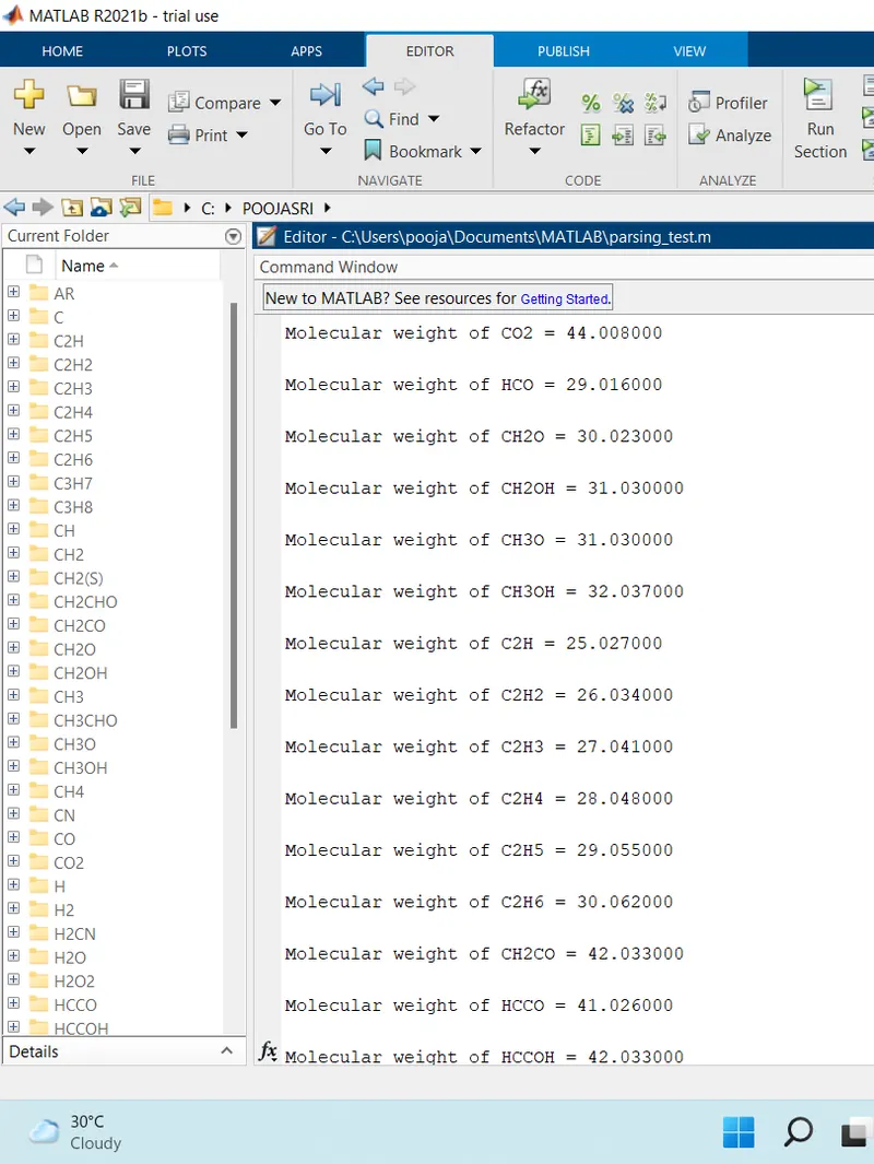
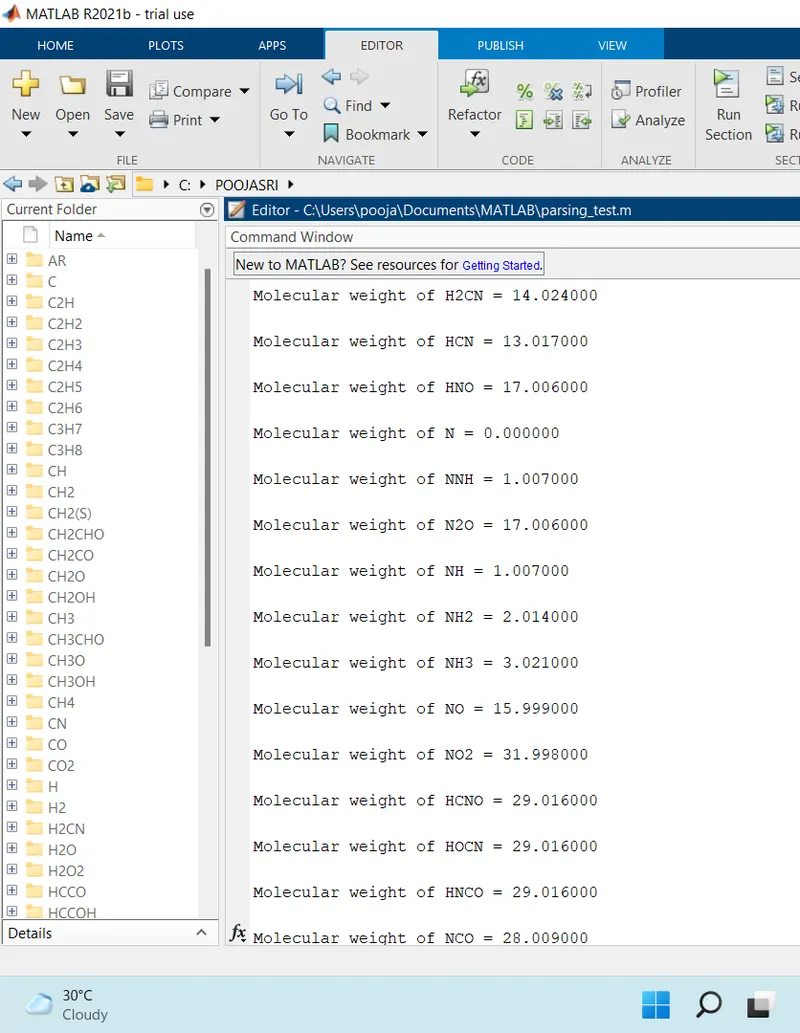
• Initializing the 'mol_weight' variable as 0.
• Creating a variable called 'elements' which contains the main elements used in the given data file.
• And creating one more variable called 'atomic_wght' which contains the atomic weight of the corresponding above elements.
• Using two for loops here, one is upto the length of the species name and one is upto the length of the above atomic_wgth.
• 'strcmp' command is used to compare the strings of species name for each iteration with the strings of elements.

ERRORS FACED WHILE PROGRAMMING :

• My plots were getting 2 curves after my first iteration completes, for further iterations also the curves were added.

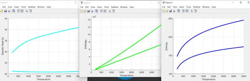
• This is because of using hold on command for all the three plots also.

CONCLUSION :

The given challenge has been acheived and the molecular weight for all the 53 species has been calculated.