Week 4.1 - Genetic Algorithm

• MATLAB CODE FOR.

1.TO OPTIMISE STALAGMITE FUNCTION.

2.TO FIND GLOBAL MAXIMA OF FUNCTION.

function [f] =stalagmite(input_vector)

x=input_vector(1);
y=input_vector(2);

f1=(sin(5.1*pi*x+0.5)).^6;
f2=exp(-4*log(2)*((x-0.0667).^2)./0.64);
f3=(sin(5.1*pi*y+0.5)).^6;
f4=exp(-4*log(2)*((y-0.0667).^2)./0.64);

f=-(f1*f2*f3*f4);
end


clear all
close all
clc

%Defining our search space

x=linspace(0,0.6,150);
y=linspace(0,0.6,150);

count=50;

%Creating 2D mesh

[xx yy] =meshgrid(x,y);

%Evaluate stalagmite function

for i=1:length(xx)
    for j=1:length(yy)
        input_vector(1)=xx(i,j);
        input_vector(2)=yy(i,j);
        f(i,j)=stalagmite(input_vector);
    end
end

tic

%Case-1- For Unbounded Inputs Variables

for i=1:count
    [inputs,foptm(i)]=ga(@stalagmite,2)
    xoptm(i)=inputs(1);
    yoptm(i)=inputs(2);
end
study1_time=toc;

%Plotting result for Case 1

subplot(2,1,1)
hold on
surfc(x,y,-f)
hold on
shading interp
xlabel('X Values')
ylabel('Y Values')
legend('X Values','Y Values')
title("Unbounded Inputs Behaviour")

hold on
plot3(xoptm,yoptm,-foptm,'Marker','o','MarkerSize',8,'MarkerFaceColor','r')
subplot(2,1,2)
plot(-foptm)
xlabel('No of Iterations')
ylabel('Maximum Function Value')

tic

%Case-2- For Bounded Inputs Variables

for i=1:count
    [inputs,foptm(i)]=ga(@stalagmite,2,[],[],[],[],[0;0],[1;1]);
    xoptm(i)=inputs(1);
    yoptm(i)=inputs(2);
end
study2_time=toc;

%Plotting result for Case 2

subplot(2,1,1)
hold on
surfc(x,y,-f)
hold on
shading interp
xlabel('X Values')
ylabel('Y Values')
legend('X Values','Y Values')
title("Bounded Inputs Behaviour")

hold on
plot3(xoptm,yoptm,-foptm,'Marker','o','MarkerSize',8,'MarkerFaceColor','r')
subplot(2,1,2)
plot(-foptm)
xlabel('No of Iterations')
ylabel('Maximum Function Value')

% Case-3 - Increase number of iterations

options = optimoptions('ga');
options = optimoptions (options,'PopulationSize',300);

tic

for i=1:count
    [inputs,foptm(i)]=ga(@stalagmite,2,[],[],[],[],[0;0],[1;1],[],[],options);
    xoptm(i)=inputs(1);
    yoptm(i)=inputs(2);
end

study3_time=toc;

%Plotting result for Case 2

subplot(2,1,1)
hold on
surfc(x,y,-f)
hold on
shading interp
xlabel('X Values')
ylabel('Y Values')
legend('X Values','Y Values')
title("Bounded Inputs Behaviour With Increased Population")

hold on
plot3(xoptm,yoptm,-foptm,'Marker','o','MarkerSize',8,'MarkerFaceColor','r')
subplot(2,1,2)
plot(-foptm)
xlabel('No of Iterations')
ylabel('Maximum Function Value')

• OUTPUT PLOTS SHOWING RESULTS

RESULT FOR CASE - 1

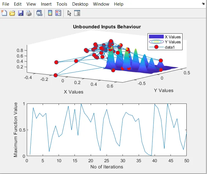
RESULT FOR CASE - 2

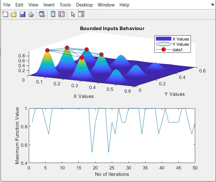
RESULT FOR CASE - 3

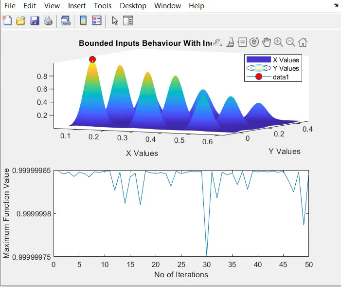
• MATLAB CODE EXPLAINATION

Code for Stalagmite Fuction to be used

function [f] =stalagmite(input_vector) Explaination : Syntax for 'stalagmite' function to be define.

x=input_vector(1); Explaination : Defining vectors for respective variables
y=input_vector(2);

Explaination : Here function follows mathematical formula to find global maxima.

f1=(sin(5.1*pi*x+0.5)).^6;
f2=exp(-4*log(2)*((x-0.0667).^2)./0.64);
f3=(sin(5.1*pi*y+0.5)).^6;
f4=exp(-4*log(2)*((y-0.0667).^2)./0.64);

f=-(f1*f2*f3*f4);Explaination : Mathematical formula to find global maxima.
end

Code for Evaluate Stalagmite Fuction

clear all
close all
clc

Explaination :Defining our search space

x=linspace(0,0.6,150);
y=linspace(0,0.6,150);

count=50; Explaination :Number of iterations to be performed

[xx yy] =meshgrid(x,y); Explaination :Creating 2D vectors

Explaination :Evaluate stalagmite function for vector inputs given.

for i=1:length(xx)
for j=1:length(yy)
input_vector(1)=xx(i,j);
input_vector(2)=yy(i,j);
f(i,j)=stalagmite(input_vector);
end
end

tic Explaination :Records running time.

%Case-1- For Unbounded Inputs Variables

for i=1:count Explaination: Looping for 50 iterations
[inputs,foptm(i)]=ga(@stalagmite,2) Explaination : Finds local maximum to function for 2 variables
xoptm(i)=inputs(1); Explaination: Inputs to variables
yoptm(i)=inputs(2);
end

study1_time=toc; Explaination :Read/Calculate elapsed time.

Explaination :Plotting result for Case 1 with all necessary information to display

subplot(2,1,1)
hold on
surfc(x,y,-f) Explaination : 3D dimentional graph
hold on
shading interp Explaination : Shading effect to 3D plots
xlabel('X Values')
ylabel('Y Values')
legend('X Values','Y Values')
title("Unbounded Inputs Behaviour")

hold on
plot3(xoptm,yoptm,-foptm,'Marker','o','MarkerSize',8,'MarkerFaceColor','r') Explaination : Plot 3D points in a 3D space
subplot(2,1,2)
plot(-foptm) Explaination : Plot maxima value in 2D graph
xlabel('No of Iterations')
ylabel('Maximum Function Value')

tic Explaination :Records running time.

%Case-2- For Bounded Inputs Variables

for i=1:count
[inputs,foptm(i)]=ga(@stalagmite,2,[],[],[],[],[0;0],[1;1]); Explaination : Finds local maximum to function for bounded 2 variables so that result will be between bounded region
xoptm(i)=inputs(1);
yoptm(i)=inputs(2);
end
study2_time=toc; Explaination :Read/Calculate elapsed time.

Explaination :Plotting result for Case 2 with all necessary information to display

subplot(2,1,1)
hold on
surfc(x,y,-f) Explaination : 3D dimentional graph
hold on
shading interp Explaination : Shading effect to 3D plots
xlabel('X Values')
ylabel('Y Values')
legend('X Values','Y Values')
title("Bounded Inputs Behaviour")

hold on
plot3(xoptm,yoptm,-foptm,'Marker','o','MarkerSize',8,'MarkerFaceColor','r') Explaination : Plot 3D points in a 3D space
subplot(2,1,2)
plot(-foptm) Explaination : Plot maxima value in 2D graph
xlabel('No of Iterations')
ylabel('Maximum Function Value')

% Case-3 - Increase number of iterations

options = optimoptions('ga'); Explaination : Solver returns sets a default options for it.
options = optimoptions (options,'PopulationSize',300); Explaination : Returns a copy of old options with parameters.

tic Explaination :Records running time.

for i=1:count
[inputs,foptm(i)]=ga(@stalagmite,2,[],[],[],[],[0;0],[1;1],[],[],options);Explaination : Finds solution to function for linear equalities constrains and boundary defined
xoptm(i)=inputs(1);
yoptm(i)=inputs(2);
end

study3_time=toc;Explaination :Read/Calculate elapsed time.

Explaination :Plotting result for Case 3 with all necessary information to display

subplot(2,1,1)
hold on
surfc(x,y,-f) Explaination : 3D dimentional graph
hold on
shading interp Explaination : Shading effect to 3D plots
xlabel('X Values')
ylabel('Y Values')
legend('X Values','Y Values')
title("Bounded Inputs Behaviour With Increased Population")

hold on
plot3(xoptm,yoptm,-foptm,'Marker','o','MarkerSize',8,'MarkerFaceColor','r') Explaination : Plot 3D points in a 3D space
subplot(2,1,2)
plot(-foptm) Explaination : Plot maxima value in 2D graph
xlabel('No of Iterations')
ylabel('Maximum Function Value')

• THEORY OF GENETIC ALGORITHM

1.What is Genetic Algorithms

Ans.Genetic algorithms commonly used to generate high-quality solutions for optimization problems and search problems.

They are simulate the process of natural selection.

2.Why use Genetic Algorithms

Ans. a) They are Robust.

b) Provide optimisation over large space state.

c) Unlike traditional AI, they do not break on slight change in input or presence of noise.

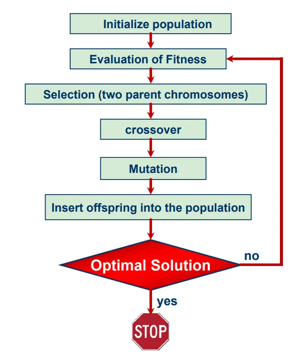
3.How Genetic Algorithms Operates

Ans. Step 1) Randomly initialize population

Step 2) Determine fitness of population

Step 3) Until convergence repeat:

a) Select parents from population

b) Crossover and generate new population

c) Perform mutation on new population

d) Calculate fitness for new population

4. Flowchart of Genetic Algorithms.

Ans.

5. Syntax of Genetic Algorithms.

Ans.

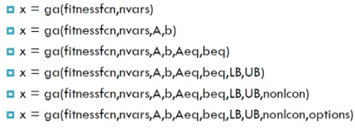
where,

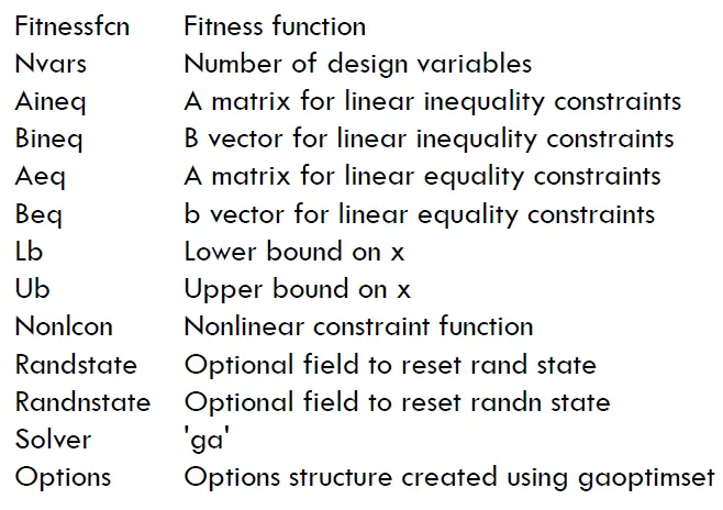
6.Significance of Iterations in Genetic Algorithms

Ans. In Genetic Algorithms, the search for the best solution depends mainly on the creation of new individuals from the old ones. The process intend to ensures the exchange of genetic material between parents and thus creates chromosomes that are more likely to be better than the parents.Thus it results into best optimised solution.