Challenge

Project 2 - Rankine cycle Simulator

SShrikant Tajane10 May 2022

1. MATLAB CODE FOR RANKINE CYCLE SIMULATOR

%% Program For Rankine Cycle Simulator

clear all
close all
clc

disp('RANKINE CYCLE');
disp('1-2 is constant pressure heat addition in the boiler');
disp('2-3 is Isentropic Expansion in the Turbine');
disp('3-4 is constant pressure heat removal in the condenser');
disp('4-1 is Isentropic compression in the pump');

p1 = input ('nValue of pressure at turbine inlet,p1(in bar)=');
T1 = input ('nValue of temperature at turbine inlet, T1(in degree.C)=');
p2 = input ('nValue of pressure at condenser inlet,p2(in bar)=');

%At State 1
h1 = XSteam('h_pT',p1,T1);
s1 = XSteam('s_pT',p1,T1);

% At State 2
s2=s1;
sf2= XSteam('sL_p',p2);
sg2= XSteam('sV_p',p2);
x2= (s2-sf2)/(sg2-sf2);
hf2= XSteam('hL_p',p2);
hg2= XSteam('hV_p',p2);
h2= hf2 + (x2*(hg2-hf2));

% At State 3
p3 = p2 ;
s3=XSteam('sL_p',p3);
h3= XSteam ('hL_p',p3);

% At State 4 
s4 = s3;
p4= p1;

%Work done by turbine
Wt = h1 -h2;

%Work done to run pump
v3 = XSteam('vL_p',p3);
Wp=v3*(p4-p3)*100;
h4= h3 + Wp;

%Net Work
Wnet = Wt - Wp;

% Heat into the system
Qin = h1 - h4 ;

% Heat out of the system
Qout = h2 -h3;

%Thermal efficiency
thermal_eff = (Wnet/Qin)*100;

%Specific Steam Consumption
%SSC = mass flow rate/power
SSC=(3600/Wnet);

%Back Work Ratio
BW = (Wp/Wt)

%Calculation of Temperature,Entropy and Enthalpy at the vapour and liquid
%line for plotting

T3 = XSteam('Tsat_p',p3);
T2=T3;
Cp4= XSteam('Cp_ps',p4,s4);
Cv4= XSteam('Cv_ps',p4,s4);
k=Cp4/Cv4;
T4=T3/((p3/p4)^((k-1)/k));

%Calculating Temperature,Entropy and Enthalpy at the vapour and liquid line
%for plotting

T6 = XSteam('Tsat_p',p1);
s5=XSteam('sL_p',p1);
s6=XSteam('sV_p',p1);
h5=XSteam('hL_p',p1);
h6=XSteam('hV_p',p1);
T5=T6;

%Plotting the saturation curve
T=linspace(1,375,1000);
for i=1:length(T)

    sf(i)=XSteam('sL_T',T(i));
    sg(i)=XSteam('sV_T',T(i));
    hf(i)=XSteam('hL_T',T(i));
    hg(i)=XSteam('hV_T',T(i));
end

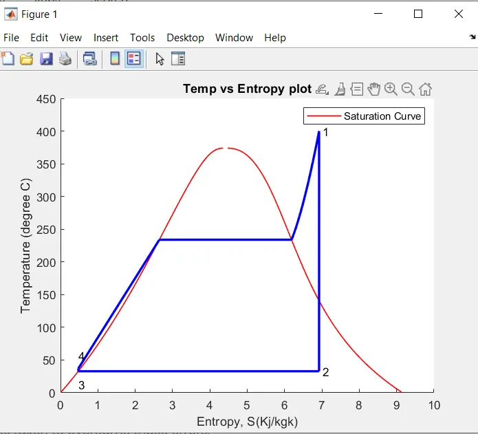
%Plotting T-s diagram
figure(1)
hold on
plot (sf,T,'r','LineWidth',1)
plot(sg,T,'r','LineWidth',1)
plot([s1 s2],[T1 T2],'b','LineWidth',2)
plot([s2 s3],[T2 T3],'b','LineWidth',2)
plot([s3 s4],[T3 T4],'b','LineWidth',2)
plot([s4 s5],[T4 T5],'b','LineWidth',2)
plot([s5 s6],[T5 T6],'b','LineWidth',2)
sc1 = linspace(s6 ,s1 , 1000);
  for l=1:length(sc1)
        Tc1(l) = XSteam ('T_ps',p1,sc1(l));
    end
    plot(sc1,Tc1,'b','LineWidth',2)
    text(s1+0.1,T1,'1')
    text(s2+0.1,T2,'2')
    text(s3,T3-20,'3')
    text(s4,T4+20,'4')
    title('Temp vs Entropy plot')
    xlabel('Entropy, S(Kj/kgk)')
    ylabel('Temperature (degree C)')
    legend('Saturation Curve')

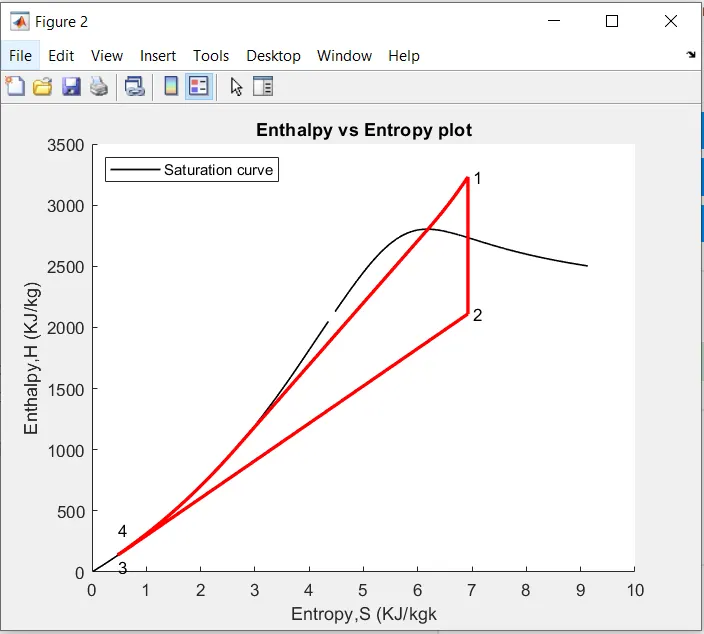
    %Plotting h-s diagram
    figure (2)
    hold on
    plot (sf,hf,'k','LineWidth',1)
    plot(sg,hg,'k','LineWidth',1)
    plot([s1 s2],[h1 h2],'r','LineWidth',2)
    plot([s2 s3],[h2 h3],'r','LineWidth',2)
    plot([s3 s4],[h3 h4],'r','LineWidth',2)
    hc = linspace (h4,h5,100);
    for r= 1:length(hc)
        sch(r) = XSteam('s_ph',p1,hc(r));
    end
    plot(sch,hc,'r','LineWidth',2)
    plot([s5 s6],[h5 h6],'r','LineWidth',2)
    for m= 1:length(sc1)
        hc1(m) = XSteam('h_ps',p1,sc1(m));
    end
    plot (sc1,hc1,'r','LineWidth',2)
    text(s1+0.1,h1,'1')
    text (s2+0.1,h2,'2')
    text(s3,h3-100,'3')
    text(s4,h4+200,'4')
    title ('Enthalpy vs Entropy plot')
    xlabel('Entropy,S (KJ/kgk')
    ylabel('Enthalpy,H (KJ/kg)')
    legend('Saturation curve','location','northwest')

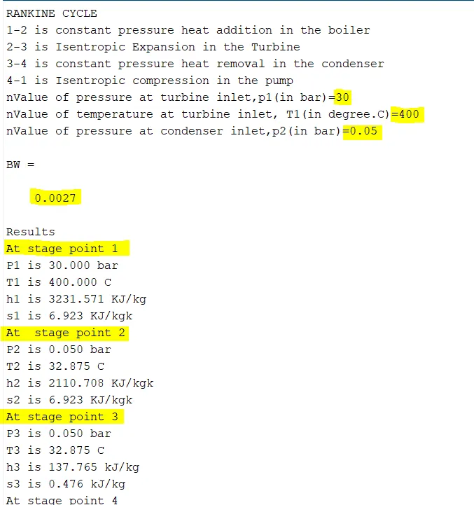
    %Displaying the results in Command window

    disp('Results');
    p1=p1;
    T1=T1;
    p2=p2;
    disp('At stage point 1');
    n1=sprintf('P1 is %.3f bar',p1);
    disp(n1);
    n2=sprintf('T1 is %.3f C',T1);
    disp(n2);
    n3=sprintf('h1 is %.3f KJ/kg',h1);
    disp(n3);
    n4=sprintf('s1 is %.3f KJ/kgk',s1);
    disp(n4);
    disp('At  stage point 2');
    n11=sprintf('P2 is %.3f bar',p2);
    disp(n11);
    n21=sprintf('T2 is %.3f C',T2);
    disp(n21);
    n31=sprintf('h2 is %.3f KJ/kgk',h2);
    disp(n31);
    n41=sprintf('s2 is %.3f KJ/kgk',s2);
    disp(n41);
    disp('At stage point 3');
    n12=sprintf('P3 is %.3f bar',p3); 
    disp(n12);
    n22=sprintf('T3 is %.3f C',T3);
    disp(n22);
    n32=sprintf('h3 is %.3f kJ/kg',h3);
    disp(n32);
    n42=sprintf('s3 is %.3f kJ/kg',s3);
    disp(n42);
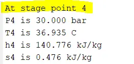
    disp('At stage point 4')
    n13 = sprintf('P4 is %.3f bar',p4);
    disp(n13);
    n23= sprintf ('T4 is %.3f C',T4);
    disp(n23);
    n33= sprintf ('h4 is %.3f kJ/kg',h4);
    disp(n33);
    n43= sprintf ('s4 is %.3f kJ/kg',s4);
    disp(n43);
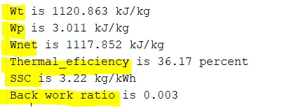
    n14= sprintf ('Wt is %.3f kJ/kg',Wt);
    disp(n14);
    n15= sprintf ('Wp is %.3f kJ/kg',Wp);
    disp(n15);
    n16= sprintf ('Wnet is %.3f kJ/kg',Wnet);
    disp(n16);
    n17= sprintf ('Thermal_eficiency is %.2f percent',thermal_eff);
    disp(n17);
    n18= sprintf ('SSC is %.2f kg/kWh',SSC);
    disp(n18);
    n19= sprintf ('Back work ratio is %.3f',BW);
    disp(n19);

2. PLOTS FOR GIVEN INPUTS.