Week 4.1 - Genetic Algorithm

1. Genetic Algorithm : 

(i)It generates a population of points at each iteration. The best point in the population approaches an optimal solution.

(ii)Selects the next population by computation which uses random number generators. It consists of three rules

a. selection

b. cross-over

c. mutation

2. Syntax for ga : 

1. x = ga(function_handle, variables)

2. x = ga(function_handle, variables, A, B, Aeq, Beq)

3. x = ga(function_handle, variables, A, B, Aeq, Beq, lb, ub, nonlcon, intcon, options)

where,

A,B = linear inequality constraints

Beq,Aeq = linear equality constraints

lb = lower bound,

ub =  upper bound,

nonlcon = non linear constraints

options =  for optimisation.

Reference : Mathworks.

3. Stalagmite Function : 

Equation of Stalagmite function : 

f= f1*f2*f3*f4,

where

f = f(x,y),

f1 = (sin(5.1*pi*x+0.5))^6,

f2 = (sin(5.1*pi*y+0.5))^6,

f3 = exp((-4*log(2)*(x-0.0067)^2)/0.64),

f4 = exp((-4*log(2)*(y-0.0067)^2)/0.64).

4. Code for Stalagmite function:

function f = stalagmite(input_vector)

x = input_vector(1);

y = input_vector(2);

f1 = (sin(5.1*pi*x+0.5))^6;
f2 = (sin(5.1*pi*y+0.5))^6;
f3 = exp((-4*log(2)*(x-0.0067)^2)/0.64);
f4 = exp((-4*log(2)*(y-0.0067)^2)/0.64);

f= f1*f2*f3*f4;
end

5. Code for Global Maxima

% Defining the search space
x = linspace(0,1,150);
y=linspace(0,1,150);

% Repition of ga
num_case = 50;

[X, Y] = meshgrid(x, y)

% calculating the function
for i = 1:length(X)
    for j = 1:length(Y)
        input_vector(1) = X(i,j);
        input_vector(2) = Y(i,j);
%         Stalagmite function uses the inputs and give the value of 'f'.
        f(i, j) = stalagmite(input_vector);
    end
end

surfc(X,Y,f);
xlabel('X axis')
ylabel('Y axis')
shading interp

tic
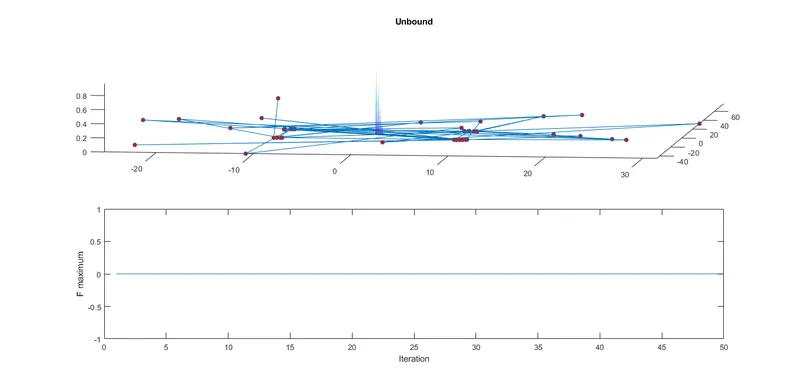
% Study for Unbounded Conditions
for i = 1:num_case
    [inputs, fopt(i)] = ga(@stalagmite,2);
%     Explanation: (i)ga is an inbuilt function 
%                  (ii)@ is used to minimise the function
%                  (iii)'2' denotes the no. of variables.
xopt(i) = inputs(1);
yopt(i) = inputs(2);
end
study1_time = toc;
% Plotting
 figure(1)
%  To create more than 1 plot we use subplot
 subplot(2,1,1)
 hold on
 surfc(x,y,f)
 shading interp %To remove the lines on the stalagmite.
 plot3(xopt, yopt, fopt, 'marker', 'o', 'markersize',5,'markerfacecolor', 'r')
 title('Unbound')
 subplot(2,1,2)
 plot(fopt)
 xlabel('Iteration');
 ylabel('F maximum');
 
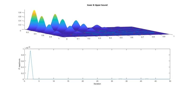
%  Study for upper and lower bound
tic
for i = 1:num_case
    [inputs, fopt(i)] = ga(@stalagmite,2, [], [], [], [], [0;0], [1;1]);
xopt(i) = inputs(1);
yopt(i) = inputs(2);
end
study2_time = toc;
% Plotting
figure(2)
 subplot(2,1,1)
 hold on
 surfc(x,y,f)
 shading interp 
 plot3(xopt, yopt, fopt, 'marker', 'o', 'markersize',5,'markerfacecolor', 'r')
 title('lower & Upper bound')
 subplot(2,1,2)
 plot(fopt)
 xlabel('Iteration');
 ylabel('F maximum');
 
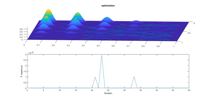
%  Study 3, Optimisation
options = optimoptions('ga')
options = optimoptions(options, 'PopulationSize',300);

tic
for i = 1:num_case
[inputs, fopt(i)] = ga(@stalagmite,2, [], [], [], [], [0;0], [1;1], [], [], options);
xopt(i) = inputs(1);
yopt(i) = inputs(2);
end
study3_time = toc;
% Plotting
figure(3)
 subplot(2,1,1)
 hold on
 surfc(x,y,f)
 shading interp 
 plot3(xopt, yopt, -fopt, 'marker', 'o', 'markersize',5,'markerfacecolor', 'r')
 title('optimisation')
 subplot(2,1,2)
 plot(fopt)
 xlabel('Iteration');
 ylabel('F maximum');