Week 4.1 - Genetic Algorithm

Aim: 1)To understand stalagmite function and its optimization methods

2)Apply genetic algorithm to get optimum results

Objective :

• Understand what is a stalagmite
• Understand Genetic algorithm

Code objective:

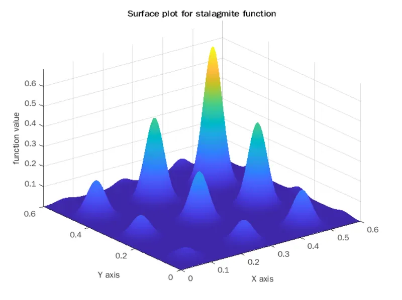
In this cod we will give values for x and y and calculate Z-axis value i.e 'f' by stalagmite function, this data will be our search space which we will

represent with the surface plot.

Then we will try to find global maxima for 'f' By 2 methods

Theory:

Stalagmite function: A stalagmite function generally refers to the function which we are generating values over stalagmite kind of surface for finding out the local and global maxima and minima of that particularly given function

Genetic algorithm :

• It is an optimization technique used to solve nonlinear optimization problems.
• It uses the concept of darwins theory of evolution to find global minima of a function

Genetic algorithm works in the following 3 steps

1) Selection: A of individuals are selected from the population in the mating pool. the best individuals are selected on basis of previous fitness value

2)Crossover: Crossover generates new offsprings by mating previously selected offsprings. The new offsprings carry genes from both parents

3)Mutation: In mutation, some selected genes are altered . it avoids falling solution into a local minima

Genetic algorithm (ga)syntax in Matlab

1)x = ga(fun,nvars) 
finds a local unconstrained minimum, x, to the objective function, 
fun. nvars is the dimension (number of design variables) of fun.

2)x = ga(fun,nvars,A,b) finds a local minimum x to fun, subject to the linear inequalities A*x ≤ b. ga evaluates the matrix product A*x as if x is transposed (A*x').


3)x = ga(fun,nvars,A,b,Aeq,beq) finds a local minimum x to fun, subject to the linear
 equalities Aeq*x = beq and A*x ≤ b. (Set A=[] and b=[] if no linear inequalities exist.) 
ga evaluates the matrix product Aeq*x as if x is transposed (Aeq*x').

4)x = ga(fun,nvars,A,b,Aeq,beq,lb,ub) defines a set of lower and upper bounds on the
 design variables, x,
 so that a solution is found in the range lb ≤ x ≤ ub. 
(Set Aeq=[] and beq=[] if no linear equalities exist.)


5)x = ga(fun,nvars,A,b,Aeq,beq,lb,ub,nonlcon) subjects the minimization to the constraints defined in nonlcon. 
The function nonlcon accepts x and returns vectors C and Ceq, representing the nonlinear inequalities and equalities respectively. ga minimizes the fun such that 
C(x) ≤ 0 and Ceq(x) = 0. (Set lb=[] and ub=[] if no bounds exist.)


6)x = ga(fun,nvars,A,b,Aeq,beq,lb,ub,nonlcon,options) minimizes with the default
 optimization parameters replaced by values in options. (Set nonlcon=[] if no nonlinear
 constraints exist.) 
Create options using optimoptions.

7)x = ga(fun,nvars,A,b,Aeq,beq,lb,ub,nonlcon,intcon) or
 x = ga(fun,nvars,A,b,Aeq,beq,lb,ub,nonlcon,intcon,options) 
requires that the variables listed in intcon take integer values.
--------------------------------------------------------------------------------------

8)x = ga(problem) finds the minimum for problem, a structure described in problem.


9)[x,fval] = ga(___), for any previous input arguments, also returns fval, 
the value of the fitness function at x.


10)[x,fval,exitflag,output] = ga(___) also returns exitflag, an integer identifying the
 reason the algorithm terminated, and output, a structure that contains output from 
each generation and other information about the performance of the algorithm.


11)[x,fval,exitflag,output,population,scores] = ga(___) also returns a matrix population, whose rows are the final population, and a vector scores, the scores of the final population.

Stalagmite Function

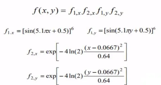
Code for stalagmite function is

%stalagmite Function
function[f]=stalagmite(inputvector)
x=inputvector(1);%acsess first coulmn of matrix input vector 
y=inputvector(2);%acsess second coulmn of matrix input vector 
f1=(sin((5.1*pi*x)+0.5)).^6;
f2=(sin((5.1*pi*y)+0.5)).^6;
f3=exp((-4*(0.6931)*(x-0.667).^2)/0.64);
f4=exp((-4*(0.6931)*(y-0.667).^2)/0.64);
f=-(f1*f2*f3*f4);%use negetive sign so that we can find maxima 

Main Code

%Stalegmite function 
clear all
close all 
clc
%defining search space
x=linspace(0,0.6,150);
y=linspace(0,0.6,150);

%Create meshgrid
[xx yy]=meshgrid(x,y);

%evaluate stalegmite function 
for i=1:length(xx)
    for j=1:length(yy)
        inputvector(1)=xx(i,j);
        inputvector(2)=yy(i,j);
        f(i,j)=stalagmite(inputvector);
    end
end
surfc(xx,yy,-f);
shading interp
xlabel('X axis')
ylabel('Y axis')
zlabel('function value')
title('Surface plot for stalagmite function' )
[inputs,fval]=ga(@stalagmite,2);
saveas(figure(1),'stalagmite figure 1','png')
num_case=50 
%----------------------------------------------------------------------------------------------
tic
%study1
for i=1:num_case
    [inputs,fopt(i)]=ga(@stalagmite,2);%here we evaluate maximum for staligmite func at 2 var x and y
    xopt(i)=inputs(1);
    yopt(i)=inputs(2);
end
study1_time=toc

%plotting for study 1
figure(2)
subplot(2,1,1)
hold on 
surfc(x,y,-f)
shading interp
plot3(xopt,yopt,-fopt,'marker','o','markersize',3,'markerfacecolor','r')
title('Unbounded inputs')
xlabel('x axis')
ylabel('y axis')
subplot(2,1,2)
plot(-fopt)
xlabel('num cases')
ylabel('f optimum')
%=============================================================================================
%study2
tic
for i=1:num_case
    [inputs,fopt(i)]=ga(@stalagmite,2,[],[],[],[],[0,0],[0.6,0.6]);
    %genetic algo solver will calc optimum f value within bounding limit x
    %and y up to 0.6 from 0
    xopt(i)=inputs(1);
    yopt(i)=inputs(2);
end
study2_time=toc

%plotting for study 2
figure(3)
hold on
subplot(2,1,1)
hold on
surfc(x,y,-f)     
shading interp
plot3(xopt,yopt,-fopt,'marker','o','markersize',3,'markerfacecolor','r')
title('Bounded inputs')
xlabel('x axis')
ylabel('y axis')
subplot(2,1,2)
plot(-fopt)
xlabel('num cases')
ylabel('f optimum')
%=======================================================================================
%study 3 
options=optimoptions('ga')
options=optimoptions(options,'populationSize',100)
tic
for i=1:num_case
    [inputs,fopt(i)]=ga(@stalagmite,2,[],[],[],[],[0,0],[0.6,0.6],[],[],options)
    xopt(i)=inputs(1);
    yopt(i)=inputs(2);
end
study3_time=toc

%plotting for study 3
figure(4)
subplot(2,1,1)
hold on 
surfc(x,y,-f)
shading interp
plot3(xopt,yopt,-fopt,'marker','o','markersize',3,'markerfacecolor','r')
title('Bounded inputs','Population size=400')
xlabel('x axis')
ylabel('y axis')
subplot(2,1,2)
plot(-fopt)
xlabel('num cases')
ylabel('f optimum')
hold off

Results

SURFACE PLOT

=======================================================================================

STUDY 1

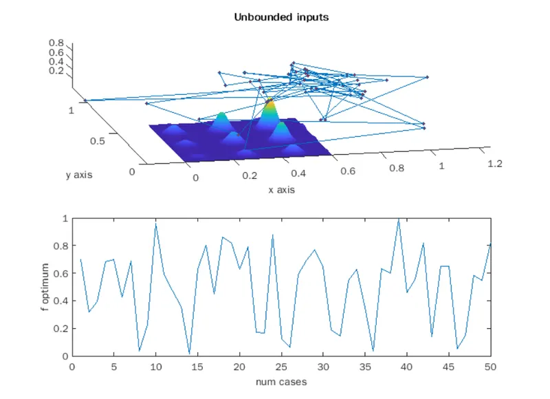
Here we get multiple co ordinates for possible maximum values for given function but we need only one i .e optimum.

=======================================================================================

STUDY 2

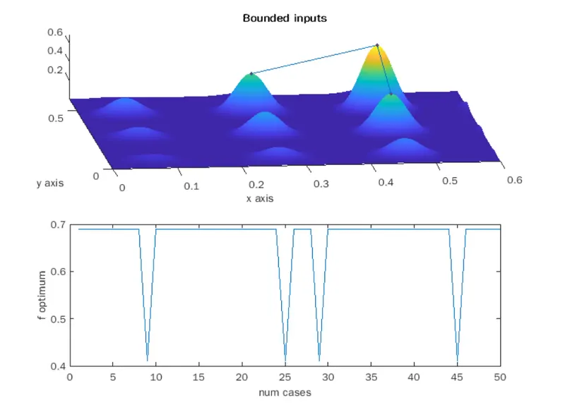
In previous study we got solutions beyond requires values of x and y so we need to set limit for x and y values

[inputs,fopt(i)]=ga(@stalagmite,2,[],[],[],[],[0,0],[0.6,0.6]);

We bounde inputs for x and y values from 0 to 0.6

But now there are 3 possible solutions , wee needd to make it more acurate

=======================================================================================

STUDY 3

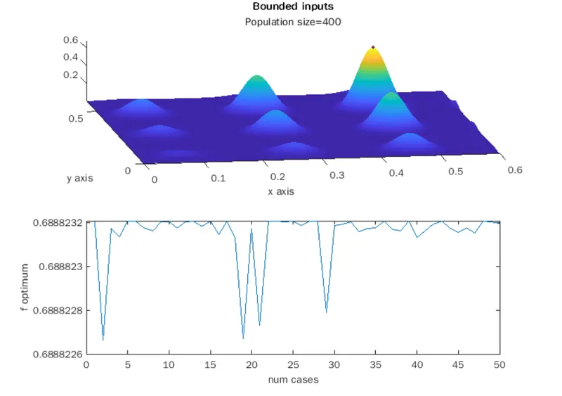
To find acurate solution we increase population size because as we know we will get more acuratet solution as population size increases for genetic algorithm

From results we can conclude that stalagmite function gives miximum value(0.6888) at xopt(0.4602) and yopt(0.4602)

=====================================================================================