Project 2 - Rankine cycle Simulator

Aim:

Create rankine cycle simulator using MATLAB

Determine h,s values at state points along the temprature range

Objective

• Determine inut values
• calculate entropy and enthalpy values for given temprature range
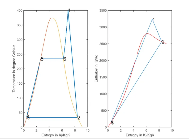
• plot t-s and h-s diagram
• create text file and write s and h values at each state

Theory:

Rankine cycle :

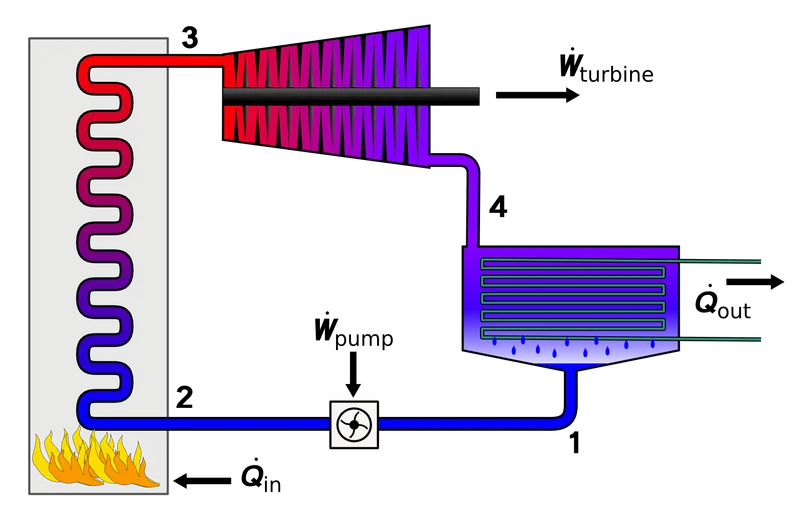
The rankine cycle is and idealised thermodynamic cycle describing the process by which certain heat engines , such as steam turbine or receprocating steam engines allow mechanical work to be exacted from a fluid as it moves between a heat source and the heat sink .

Rankine cycle is used for thermalpower genration plants where mater is pumped to moiler where it get heated to genrate steam and then this steam expand over turbine to genrate electricity ,Aftter expansion steam get condenced at normal temprature

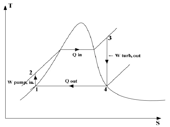
Technically there are four thermodynamic process ocur in rankine cycle.

1) Isentropic pumping of condenced fluid from condencer to boiler ,As process is isentropic tere is no heat tansfer between system and surrounding

Wpump =h2-h1

2)Constant pressure heat addition : Liqiuid water entering to boiler heated to super heated state in boiler.

qin=h3-h2

3)isentropic expansion at Turbine: Super heated steam expanded over turbine isentroicaly

Wturbine= h3-h4

4)Condensation:Steam out from turbine ge condenced at contant pressure .

qout=h4-h1

for whole cycle energy balence equation will be

(qin-qout)-(Wturbine,out-wpump,in)=0

Where net work done is

Wnet,out=Wturbine,out-Wpimp,in

close all
clear all
clc
%xsteam.m file and dounloaded to current drive
f1=fopen("Rankine cycle data.txt","w")
fprintf(f1,'1-2 Isobaric heat transfer\n')
fprintf(f1,'2-3 isentropic expansion\n')
fprintf(f1,'3-4 isobaric heat rejection\n')
fprintf(f1,'4-1 isobaric compression\n')

%inputs
p1=input('Enter the pressure at turbiine inlet(in bar):');
T1=input('Enter the temprature at turbiine inlet(in deg.celcious):');
p2=input('Enter the pressure at condensor (in bar):');

%calculating h,s,v values at each stage 
%point1
h1=XSteam('h_pt',p1,T1);
s1=XSteam('s_pt',p1,T1);

%point2
s2=s1
sf2=XSteam('sL_p',p2);
sg2=XSteam('sV_p',p2);
hf2=XSteam('hL_p',p2);
hg2=XSteam('hV_p',p2); %x2=(s2-sf2)/(sg2-sf2)
s2=sg2;
h2=hg2;                %hf2+(x2*(hg2-hf2));
T2=XSteam('T_hs',h2,s2);

%point 3
T3=T2;
p3=p2;
s3=XSteam('sL_T',T3);
h3=XSteam('hL_T',T3);
v3=XSteam('vL_p',p2);

%point 4
p4=p1;
s4=s3;
cp4=XSteam('Cp_ps',p4,s4);
cv4=XSteam('Cv_ps',p4,s4);
gamma=(cp4/cv4);
r=(gamma-1)/gamma;
T4=T3*(p4/p3)^r;

%point 5

T5=XSteam('Tsat_p',p1);
s5=XSteam('sL_P',p1);
h5=XSteam('hL_p',p1);

%point6
T6=T5
s6=XSteam('sV_P',p1);
h6=XSteam('hV_p',p1);



%Calculations

Wt=h1-h2;
Wp=v3*(p1-p2)*100;
h4=Wp+h3;
W_net= Wt-Wp;
Qs=h1-h4;
N_per=(W_net/Qs)*100;
steam_rate=3600/(Wt-Wp);



%plot T-S Diagram 
subplot(1,2,1);
T_rankine=linspace(T5,T1,5000);
for i= 1 : length(T_rankine);
    s_rankine(i)=XSteam('s_pT',p1,T_rankine(i));
end
plot([s1 s2 s3 s4 s5 s6 s_rankine],[T1 T2 T3 T4 T5 T6 T_rankine],'LineWidth',1.5);
hold on
T_curve=linspace(1,400,500);
for i=1:length(T_curve);
    s_l(i)=XSteam('sL_T',T_curve(i));
    s_v(i)=XSteam('sV_T',T_curve(i));
    h_l(i)=XSteam('hL_T',T_curve(i));
    h_v(i)=XSteam('hV_T',T_curve(i));
end

plot(s_l,T_curve);
plot(s_v,T_curve);
text(s1,T1,'1','FontSize',15);
text(s2,T2,'2','FontSize',15);
text(s3,T3,'3','FontSize',15);
text(s4,T4,'4','FontSize',15);
text(s5,T5,'5','FontSize',15);
text(s6,T6,'6','FontSize',15);
xlabel('Entropy in Kj/KgK');
ylabel('Temprature in degree Celcius');

%PLot HS Diagram 
subplot(1,2,2)
plot([s1 s2 s3 s4 s1],[h1 h2 h3 h4 h1])
hold on 
plot(s_v,h_v,'color','r')
plot(s_l,h_l,'color','r')
text(s1,h1,'1','FontSize',15);
text(s2,h2,'2','FontSize',15);
text(s3,h3,'3','FontSize',15);
text(s4,h4,'4','FontSize',15);
xlabel('Entropy in Kj/KgK');
ylabel('Enthalpy in Kj/Kg');

%write file


fprintf(f1,'\n=================Result=================\n')
fprintf(f1,'At State point 1:\nP1 is : %4.2f Bar\nT1 is :%4.3f Degree Celcius \nH1 is: %4.2f KJ/Kg \nS1 is : 4.2f Kj/Kg.k ',p1,T1,h1,s1);
fprintf(f1,' \n');
fprintf(f1,'At State point 2:\nP2 is : %4.2f Bar\nT2 is :%4.3f Degree Celcius \nH2 is: %4.2f KJ/Kg \nS2 is : 4.2f Kj/Kg.k ',p2,T2,h2,s2);
fprintf(f1,' \n');
fprintf(f1,'At State point 3:\nP3 is : %4.2f Bar\nT3 is :%4.3f Degree Celcius \nH3 is: %4.2f KJ/Kg \nS3 is : 4.2f Kj/Kg.k ',p3,T3,h3,s3);
fprintf(f1,'\n');
fprintf(f1,'At State point 4:\nP4 is : %4.2f Bar\nT3 is :%4.3f Degree Celcius \nH4 is: %4.2f KJ/Kg \nS4 is : 4.2f Kj/Kg.k ',p4,T3,h4,s4);
fprintf(f1,' \n');
fprintf(f1,'Wt is :%4.2f Kj/Kg\nWp is: %4.2f Kj/Kg\nWnet is : %4.2f KjKg \nNtherm is : %4.2f Kg/KWh',Wt,Wp,W_net,N_per);   
fclose(f1)

Results

T-S Diagram T-H Diagram

Text file data :