Week 3 - Solving second order ODEs

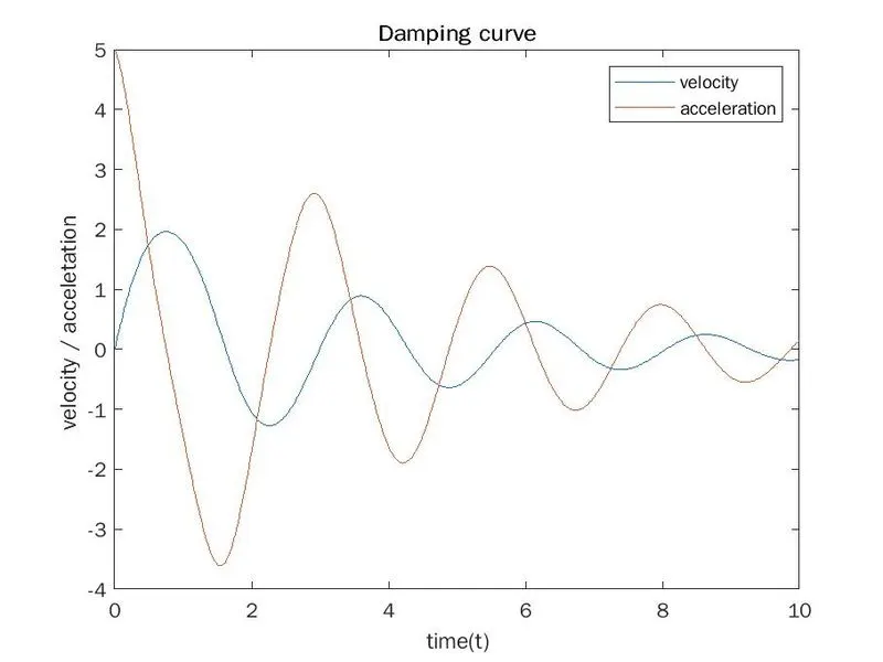
Aim: 1)To write a program to plot angular velocity and acceleration curve VS time 

        2)To write a program to simulate motion of pendulum

Objective :

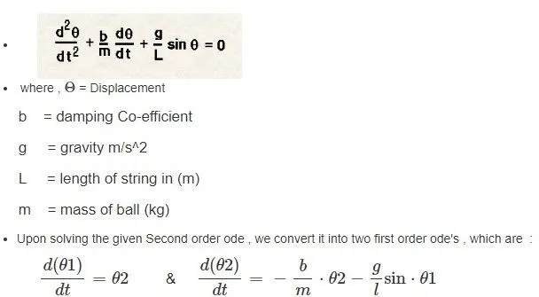
1)Understand spring damping eqn 

2)Convert second order diffrential eqn iin to first order diffrential eqn 

3)genrate function (ode_func) for ordinary eqn's 

4) Write a program using 'ode45'to solve the eqn's to find theta at time t

5)Simulate pendulum using theta values

Theory:

Secondary differential eqn's are widly used in various engineering applications here we are using spring damping eqn 

                                    

Function Code:

function [dtheta_dt]=ode_func(t,theta,b,g,l,m)   %define function
theta1=theta(1)                                  %access thta1 matrix values
theta2=theta(2)                                  %access thta1 matrix values
dtheta1_dt=theta2;                               %
dtheta2_dt=-(b/m).*theta2-(g/l).*sin(theta1);    %framing eqn in matlab 
dtheta_dt=[dtheta1_dt;dtheta2_dt];
end

Main Code:

% clc
clear all
close all
%Solve ODE for Pendulam 
b=0.5                       %damping coifficient
g=9.81                      
l=1.5                       %length of string                       
m=1                         %mass
theta_0=[0;5]               %initial velicity;acceleration
t_span=linspace(0,10,500)   %time span                      

%%
%solve ode
[t,results]=ode45(@(t,theta)ode_func(t,theta,b,g,l,m),t_span,theta_0);

plot(t,results(:,1))         %plot at vs vlues of result matrix all rows first column
hold on 
plot(t,results(:,2))
legend('velocity','acceleration')
hold off
title('Damping curve')
xlabel('time(t)')
ylabel('velocity / acceletation ')



%to create simulation of pendulam osscilation and damping
theta=results(:,1);
ct=1                             %conter for counting frames
for i=1:length(theta);
    Theta=theta(i);
    %initial points
    x0=0                         %plot hinged end of string
    y0=0                         
    l=1.5                        %length
    x1=l*sin(Theta)              %plotting onother end for eac loop
    y1=-l*cos(Theta)
    figure(2)
plot([x0 x1],[y0 y1],'linewidth',3,'color','g')
hold on 
plot(x1,y1,'o','markersize',20,'markerfacecolor','r')
plot(0,0,'o','markersize',15,'markerfacecolor',[ 0 0 0])    
line([-0.5 0.5],[0 0],'linewidth',5,'color',[0 0 0])
title('Pendulum Oscillation Simulation','for damp coif=0.5 m=1')
hold off

axis([-2 2 -2 2])
pause(0.001)

M(ct)=getframe(gcf);
ct=ct+1

end
movie(M)
videofile=VideoWriter('pendulam osscilation simulation ','uncompressed AVI')
open(videofile)
writeVideo(videofile,M)
close(videofile)

 Results

Damping curve Plot:

                         

Pendulum osscilation Simulation: