Week 4.1 - Genetic Algorithm
OBJECTIVE - Write a code in MATLAB to optimise the stalagmite function and find the global maxima of the function.
THEORY:
DEFINITION:
GENETIC ALGORITHM is a search heuristic that is inspired by Charles Darwin theory of natural evolution.This algorithm reflects the process of natural selection where the fittest individuals are selected for reproduction to generate offsprings for the next generation.
PROCESS OF NATURAL SELECTION:
This process starts with the selection of the fittest individual from a given set of population.
They produce offsprings who inherit the characteristic of the parents and will be added to the next generation.
If the parents are fit enough, their offsprings will be better than their parents and will have better chances of surviving.
This process keeps on iterating and in the end, a generation of fittest individuals will be obtained.
This whole notion can be helpful in search problems.
We select a set of solutions to a problem and sort out a set of best ones out of them. This will eventually narrow down to one best solution that gives optimum results for the given problem.
There are five phases in the genetic algorithm and are explained as below:
1.) Initial population
The problem initiates with a set of individuals which is called population. Each individual is a solution to the problem we want to solve.
Each individual is characterized by a set of parameters called genes.
Genes are joined into a string which yields us chromosome which is nothing but a solution.
2.)FITNESS FUNCTION:
The fitness function determines how to fit an individual is. It gives a fitness score to each individual.
The probability that an individual will be selected for reproduction is based on this score.
3.)SELECTION PHASE
The main objective of this phase is to select the fittest individual and let them pass their Gene onto the next generation.
4.)CROSSOVER
For each pair of parents to be mated, the crossover point is chosen at random from within the genes.
For example, consider the crossover point to be 3 as in the figure below:
Offsprings are created by exchanging genes of parents among themselves until the crossover point is reached.
5.)MUTATION
In certain new offsprings formed, some of their genes can be subjected to mutation with low random probability.
This implies that some of the bits in the bit string can be flipped.
Mutation occurs to maintain diversity within the population and prevent premature convergence.
PROGRAM FOR GENETIC ALGORITHM IN MATLAB:
1.)The first code below defines the stalagmite function that will be called in the main function.
function [F] = stalagmite(input_vector)
         x=input_vector(1) ;
         y=input_vector(2) ;

         f1_x = (sin(5.1*pi*x+0.5)).^6;
         f1_y = (sin(5.1*pi*y+0.5)).^6;
         f2_x = exp(-4*log(2)*((x-0.0667).^2)/0.64);
         f2_y = exp(-4*log(2)*((y-0.0667).^2)/0.64);
         [F] = -(f1_x.*f1_y.*f2_x.*f2_y);
         end
i.) The above function defines the stalagmite function which will be used in the main function.
ii.) The input vectors 'x' and 'y' will be assigned with the required values in the main function.
iii.) The negative sign used in the last line is used to maximize the stalagmite function.
Stepwise explanation of the program:
i.) First, the search space required to execute the program is defined which varies from 0 to 0.6 with 150 divisions in between.
ii.)using the mesh grid command, row vectors x and y are converted into matrices xx and yy.
iii.) With the help of for loop, the input vectors required for the stalagmite function are defined using the matrices xx and yy.
From here onwards, the whole program is divided into three iterations and will be made to run individually:
1st iteration:
2.) The main code below uses the stalagmite function defined to find the global maxima using MATLAB's in-built 'ga' function:
% Step 1
% clearing workspace, command window & closing all plots
close all
clear all
clc

% Step 2
% Define our search space
x = linspace(0,0.6,150);
y = linspace(0,0.6,150);

% Step 3
% Calculating a 2Dimentionl mesh
[xx, yy] = meshgrid(x,y);

% Step 4
%Evaluating the stalagmite function
for i = 1:length(xx)
    for j = 1:length(yy)
        input_vector(1) = xx(i,j);
        input_vector(2) = yy(i,j);
        f(i,j) = stalagmite(input_vector);
    end
end

tic
% Step 5
% Study1- Statical behaviar
num_cases =  50;
for i=1:num_cases
    [inputs, fopt(i)] = ga(@stalagmite,30);
    xopt(i) = inputs(1);
    yopt(i) = inputs(2);
end
study1_time = toc
F=-f;
figure(1)
subplot(2,1,1)
hold on
surfc(x, y, F)
shading interp
plot3(xopt,yopt,-fopt,'marker','o','markersize',5,'markerfacecolor','r')
title('Unbounded inputs')
xlabel('x')
ylabel('y')
zlabel('f')
subplot(2,1,2)
plot(-fopt)
xlabel('Iterations')
ylabel('Function maximum')
Result:
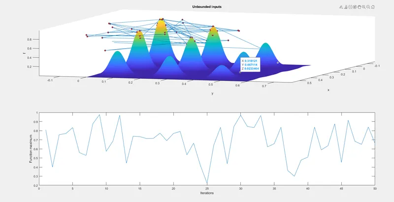
1st iteration:
In the first iteration, the behaviour of the algorithm is studied by not defining the limits.
case 2
2nd iteration:
Here the limits i.e., the lower and upper bounds are defined so as to know the boundaries within which the global maxima lies.
% Step 1
% clearing workspace, command window & closing all plots
close all
clear all
clc

% Step 2
% Define our search space
x = linspace(0,0.6,150);
y = linspace(0,0.6,150);

% Step 3
% Calculating a 2Dimentionl mesh
[xx, yy] = meshgrid(x,y);

% Step 4
%Evaluating the stalagmite function
for i = 1:length(xx)
    for j = 1:length(yy)
        input_vector(1) = xx(i,j);
        input_vector(2) = yy(i,j);
        f(i,j) = stalagmite(input_vector);
    end
end

% Step 6
% Study2- Statical buhaviour with upper and lover bounds
options = optimoptions('ga','populationSize',50);
tic
num_cases =  50;
for i = 1:num_cases
    [inputs,fopt(i)] = ga(@stalagmite,2,[],[],[],[],[0;0],[0.6;0.6]);
    xopt(i) = inputs(1);
    yopt(i) = inputs(2);
end
Study2_time = toc
figure(2)
F=-f;
subplot(2,1,1)
hold on
surfc(x, y, F)
shading interp
plot3(xopt,yopt,-fopt,'marker','o','markersize',5,'markerfacecolor','r')
title('Bounded inputs')
xlabel('x')
ylabel('y')
zlabel('f')
subplot(2,1,2)
plot(-fopt)
xlabel('Iterations')
ylabel('Function Maximum')
Result:
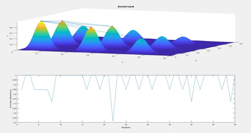
3rd iteration:
In the next step, the population size is increased so as to converge to the global maxima.
% Step 1
% clearing workspace, command window & closing all plots
close all
clear all
clc

% Step 2
% Define our search space
x = linspace(0,0.6,150);
y = linspace(0,0.6,150);

% Step 3
% Calculating a 2Dimentionl mesh
[xx, yy] = meshgrid(x,y);

% Step 4
%Evaluating the stalagmite function
for i = 1:length(xx)
    for j = 1:length(yy)
        input_vector(1) = xx(i,j);
        input_vector(2) = yy(i,j);
        f(i,j) = stalagmite(input_vector);
    end
end

% Step 7
% Study3- Increasing GA iteration
options = optimoptions('ga','populationSize',200);
tic
num_cases =  50;
for i = 1:num_cases
    [inputs, fopt(i)] = ga(@stalagmite,2,[],[],[],[],[0;0],[0.6;0.6],[],[],...
        options);
    xopt(i) = inputs(1);
    yopt(i) = inputs(2);
end
study3_time = toc
figure(3)
F=-f;
subplot(2,1,1)
hold on
surfc(x, y, F)
shading interp
plot3(xopt,yopt,-fopt,'marker','o','markersize',5,'markerfacecolor','r')
title('Bounded inputs with modified population size')
xlabel('x')
ylabel('y')
zlabel('f')
subplot(2,1,2)
plot(-fopt)
axis([0 50 0 1.5]);
xlabel('Iterations')
ylabel('Function Maximum')
FMAX=-min(fopt);
X=mean(xopt);
Y=mean(yopt);
Result:
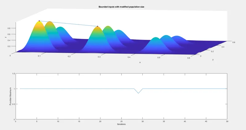
ga syntax explaination:
The format for writing a genetic algorithm in Matlab is as follows:
f_min = ga(@function,nvars,A,B,Aeq,Beq,LB,UB,nonlcon,intcon,options)
Explanation of terms involved:
- f_min is the local minima point.
- @function is the function to be called. (In our case, its the stalagmite function)
- nvars indicates the no of variables used.
- A and B are used to indicate any kind of inequalities that exist in the function.
- Same goes with Aeq and Beq.
- LB = lower bound.
- UB = upper bound.
- nonlcon gives two vectors representing inequalities and equalities.
- options are used to perform additional operations like increasing population size. This is done with the help of optic options