Week 4.1 - Genetic Algorithm
Aim: Write a code in MATLAB to optimise the stalagmite function and find the Global Maxima of the function.
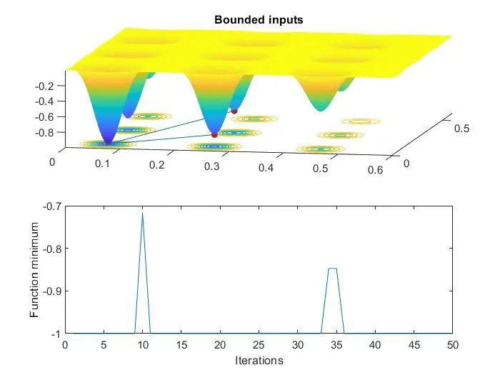
Question asaked in video the meaning of ga(@stalagmite,2,[],[],[],[],[0;0],[1;1]);
answer:
GA
Find minimum of function using genetic algorithm
Sytax:
Description
x = ga(fun,nvars)x, to the objective function, fun. nvars is the dimension (number of design variables) of fun.
Note
Passing Extra Parameters explains how to pass extra parameters to the objective function and nonlinear constraint functions, if necessary.
x = ga(fun,nvars,A,b,Aeq,beq,lb,ub,nonlcon)nonlcon. The function nonlcon accepts x and returns vectors C and Ceq, representing the nonlinear inequalities and equalities respectively. ga minimizes the fun such that C(x) ≤ 0 and Ceq(x) = 0. (Set lb=[] and ub=[] if no bounds exist.)
x = ga(fun,nvars,A,b,Aeq,beq,lb,ub,nonlcon,intcon)x = ga(fun,nvars,A,b,Aeq,beq,lb,ub,nonlcon,intcon,options)intcon take integer values.
Note
When there are integer constraints, ga does not accept nonlinear equality constraints, only nonlinear inequality constraints.
[ also returns a matrix x,fval,exitflag,output,population,scores] = ga(___)population, whose rows are the final population, and a vector scores, the scores of the final population.
Code:
clear all
close all
clc
%Defining our search space
x=linspace(0,0.6,150);
y=linspace(0,0.6,150);
num_cases=50;
%Creating a dimensional mesh
[xx yy]=meshgrid(x,y);
%Evaluating stalagmite function
for i=1:length(xx)
for j=1:length(yy)
input_vector(1)=xx(i,j);
input_vector(2)=yy(i,j);
f(i,j)=stalagmite(input_vector);
end
end
tic
% Study 1 - statistical Behaviour
for i=1:num_cases
[inputs,fopt(i)]=ga(@stalagmite,2);
xopt(i)=inputs(1);
yopt(i)=inputs(2);
end
study1_time=toc;
figure(1)
subplot(2,1,1)
hold on
surfc(x,y,f)
shading interp
plot3(xopt,yopt,fopt,'marker','O','MarkerSize',5,'MarkerFaceColor','r')
title('Unbounded inputs')
subplot(2,1,2)
plot(fopt)
xlabel('Iterations')
ylabel('Function minimum')
tic
% Study 2 - Statistical behaviour with with upper and lower bounds
for i=1:num_cases
[inputs,fopt(i)]=ga(@stalagmite,2,[],[],[],[],[0;0],[1;1]);
xopt(i)=inputs(1);
yopt(i)=inputs(2);
end
study2_time=toc;
figure(2)
subplot(2,1,1)
hold on
surfc(x,y,f)
shading interp
plot3(xopt,yopt,fopt,'marker','O','MarkerSize',5,'MarkerFaceColor','r')
title('Bounded inputs')
subplot(2,1,2)
plot(fopt)
xlabel('Iterations')
ylabel('Function minimum')
%Study 3 increasing GA iterations
options=optimoptions('ga');
options=optimoptions(options,'PopulationSize',170);
tic
for i=1:num_cases
[inputs,fopt(i)]=ga(@stalagmite,2,[],[],[],[],[0;0],[1;1],[],[],options);
xopt(i)=inputs(1);
yopt(i)=inputs(2);
end
study3_time=toc;
figure(3)
subplot(2,1,1)
hold on
surfc(x,y,f)
shading interp
plot3(xopt,yopt,fopt,'marker','O','MarkerSize',5,'MarkerFaceColor','r')
title('Bounded inputs')
subplot(2,1,2)
plot(fopt)
xlabel('Iterations')
ylabel('Function minimum')
Stalagmite function code:
function f=stalagmite(input_vector)
x=input_vector(1);
y=input_vector(2);
f1=(sin(5.1*pi*x+0.5)).^6;
f2=(sin(5.1*pi*y+0.5)).^6;
f3=exp(-4*log(2)*((x-0.0667).^2)/0.64);
f4=exp(-4*log(2)*((y-0.0667).^2)/0.64);
f=-(f1*f2*f3*f4);
end
Code explaination:
First we started with as always
clear all
close all
clc
Then we defining x and values and also number of cases in 50 values.
x=linspace(0,0.6,150);
y=linspace(0,0.6,150);
num_cases=50;
Then we creating 2 dimensional mesh with the help of meshgrid function.
%Creating a dimensional mesh
[xx yy]=meshgrid(x,y);
for i=1:length(xx)
for j=1:length(yy)
input_vector(1)=xx(i,j);
input_vector(2)=yy(i,j);
f(i,j)=stalagmite(input_vector);
end
end
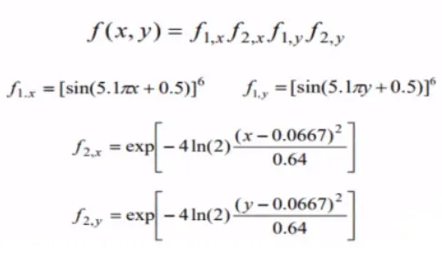
After that we evaluating the stalagmite function. In this the stalagmite function formula is converted into a code.
Formula
Code:
function f=stalagmite(input_vector)
x=input_vector(1);
y=input_vector(2);
f1=(sin(5.1*pi*x+0.5)).^6;
f2=(sin(5.1*pi*y+0.5)).^6;
f3=exp(-4*log(2)*((x-0.0667).^2)/0.64);
f4=exp(-4*log(2)*((y-0.0667).^2)/0.64);
f=-(f1*f2*f3*f4);
end
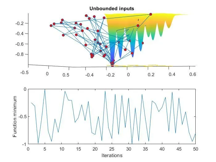
Now we are making our first study-
tic
% Study 1 - statistical Behaviour
for i=1:num_cases
[inputs,fopt(i)]=ga(@stalagmite,2);
xopt(i)=inputs(1);
yopt(i)=inputs(2);
end
study1_time=toc;
figure(1)
subplot(2,1,1)
hold on
surfc(x,y,f)
shading interp
plot3(xopt,yopt,fopt,'marker','O','MarkerSize',5,'MarkerFaceColor','r')
title('Unbounded inputs')
subplot(2,1,2)
plot(fopt)
xlabel('Iterations')
ylabel('Function minimum')
In this we are taking number of iterations = num_cases and we are using genetic algorithm function to find the maxima.
in this we calculate the study_time by using tic toc command.
we store the inputs into xopt and yopt and fopt is the optimun value at which we get the maxima.
Now we need to plot a surface of x,y and f to get the 3D plot. In this we use shading interp function to get plain plot.
We use plot3 command to plot xopt,yopt and fopt to plot optimum maximas.
We also plot for fopt to visualise the each values at each iteration and to get a maximum value.
Now we are making second study in between bounded points.
tic
% Study 2 - Statistical behaviour with with upper and lower bounds
for i=1:num_cases
[inputs,fopt(i)]=ga(@stalagmite,2,[],[],[],[],[0;0],[1;1]);
xopt(i)=inputs(1);
yopt(i)=inputs(2);
end
study2_time=toc;
figure(2)
subplot(2,1,1)
hold on
surfc(x,y,f)
shading interp
plot3(xopt,yopt,fopt,'marker','O','MarkerSize',5,'MarkerFaceColor','r')
title('Bounded inputs')
subplot(2,1,2)
plot(fopt)
xlabel('Iterations')
ylabel('Function minimum')
In this also we are taking number of iterations = num_cases and we are using genetic algorithm function.
in this we also calculate the study2_time.
we store the inputs into xopt and yopt and fopt is the optimun value at which we get the maxima.
Now we need to plot a surface of x,y and f to get the 3D plot. In this we use shading interp function to get plain plot.
We use plot3 command to plot xopt,yopt and fopt to plot optimum maximas.
We also plot for fopt to visualise the each values at each iteration and to get a maximum value.
Now we are making third study
%Study 3 increasing GA iterations
options=optimoptions('ga');
options=optimoptions(options,'PopulationSize',170);
tic
for i=1:num_cases
[inputs,fopt(i)]=ga(@stalagmite,2,[],[],[],[],[0;0],[1;1],[],[],options);
xopt(i)=inputs(1);
yopt(i)=inputs(2);
end
study3_time=toc;
figure(3)
subplot(2,1,1)
hold on
surfc(x,y,f)
shading interp
plot3(xopt,yopt,fopt,'marker','O','MarkerSize',5,'MarkerFaceColor','r')
title('Bounded inputs')
subplot(2,1,2)
plot(fopt)
xlabel('Iterations')
ylabel('Function minimum')
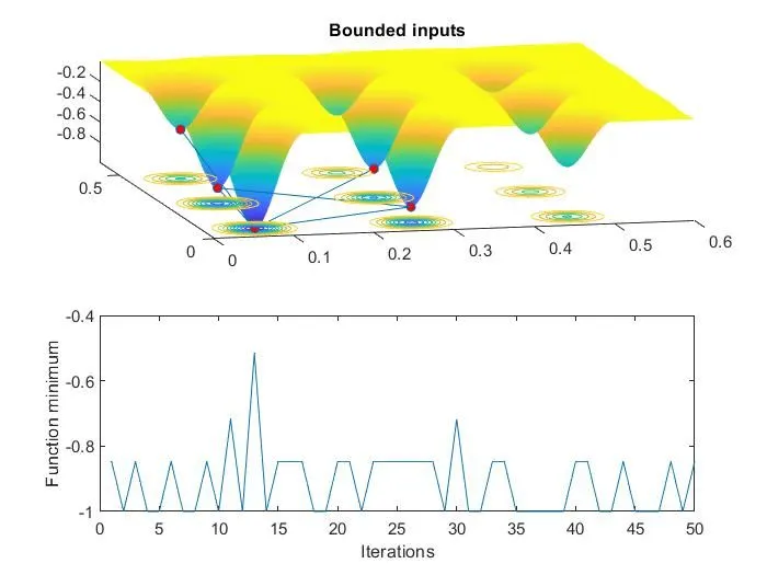
In this we are increasing population size to 170 and to get the initial population we use 'optimoptions' command
In this also we are taking number of iterations = num_cases and we are using genetic algorithm function.
in this we also calculate the study3_time.
we store the inputs into xopt and yopt and fopt is the optimun value at which we get the maxima.
Now we need to plot a surface of x,y and f to get the 3D plot. In this we use shading interp function to get plain plot.
We use plot3 command to plot xopt,yopt and fopt to plot optimum maximas.
We also plot for fopt to visualise the each values at each iteration and to get a maximum value.