Week 3 - Solving second order ODEs
Aim: Solving second order ODE
In Engineering, ODE is used to describe the transient behavior of a system. A simple example is a pendulum
The way the pendulum moves depends on the Newtons second law. When this law is written down, we get a second order Ordinary Differential Equation that describes the position of the "ball" w.r.t time.
Second order differential equation is,
In the above equation,
g = gravity in m/s2,
L = length of the pendulum in m,
m = mass of the ball in kg,
b=damping coefficient.
Given:
L=1 metre,
m=1 kg,
b=0.05.
g=9.81 m/s2.
Simulate the motion between 0-20 sec, for angular displacement=0,angular velocity=3 rad/sec at time t=0.
In this we are going to write a program in Matlab\Octave that will simulate the pendulum motion.
Program:
clear all
close all
clc
%Inputs
b=0.05; % damping coefficient
g=9.81; % gravity in m/s2
l=1; % length of the pendulum in m
m=0.1; % mass of the ball in kg
%Initial conditions
theta_0=[0;3];
%Time points
t_span=linspace(0,20,500);
%solve ODE
[t,results]=ode45(@(t,theta) ode_func(t,theta,b,g,l,m),t_span,theta_0);
%plot
%Pendulum
count=1;
for i=1:length(results(:,1));
x0=0;
y0=0;
x1=-l*sin(results(i,1));
y1=-l*cos(results(i,1));
plot([-0.5,0.5],[0,0],'LineWidth',3);
line([x0,x1],[y0,y1],'linewidth',3);
hold on
plot(x1,y1,'O','markers',20,'markerfacecolor','r');
grid on
axis([-2 2 -2 1]);
pause(0.01);
hold off
M(count)=getframe(gcf);
count=count+1;
end
movie(M)
videofile=VideoWriter('pendulum1.avi','Uncompressed AVI')
open(videofile)
writeVideo(videofile,M)
close(videofile)
ODE function program:
function [dtheta_dt]=ode_func(t,theta,b,g,l,m)
theta1=theta(1);
theta2=theta(2);
dtheta1_dt=theta2;
dtheta2_dt=-(b/m)*theta2-(g/l)*sin(theta1);
dtheta_dt=[dtheta1_dt;dtheta2_dt];
end
Code explaination:
As like every time we are staritng our program with clear all , close all, clc.
In this program we are defined the inputs of the differential equation are damping coefficient(b),gravity(g),length of the pendulum(l) and mass of the ball(m) and also there values are given in the problem.
After this we are giving initial condition like angular displacement and angular velovity with variable theta_0 and also we are giving time span of 0 to 20 as it is given 500 values.
Then we are solving the second order differential equation as given in the code. The ode45 is inbuilt differential equation
is used to differntiate the function. Then we define our ode function followed by t_span and theta_0. By this we are getting column matrices having two values.
The ode_func is the modification of this formula into the code:
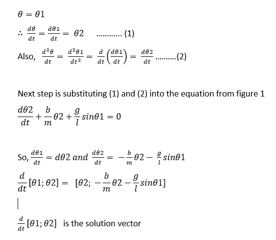
Then we are using for loop to calculate the motion of pendulum at different time intervals and position of the pendulum is calculated using the formulas
x1=-l*sin(results(i,1))
y1=-l*cos(results(i,1))
Markers command is used to create the ball
getframe(gcf) is used to get all the images at every point.
And at last we creating a movie using movie command.
Video link: