Week 4.1 - Genetic Algorithm

clear all
close all
clc 
x=linspace(0,0.6,150);
y=linspace(0,0.6,150);
num_cases=50
[xx yy]=meshgrid(x,y);
for i=1:length(xx)
    for j=1:length(yy)
        input_vector(1)=xx(i,j);
        input_vector(2)=yy(i,j);
        f(i,j)=stalagamite(input_vector);
    end
end

%  study 1 ststistical behaviour
for i=1:num_cases
    [inputs,fopt(i)]=ga(@stalagamite,2);
    xopt(i)=inputs(1);
    yopt(i)=inputs(2);
end
figure(1)
subplot(2,1,1)
hold on
surfc(x,y,f)
shading interp
plot3(xopt,yopt,fopt,'marker','o','markersize',5,'markerfacecolor','r')
xlabel('x value')
ylabel('y value')
title('unbounded inputs')
subplot(2,1,2)
plot(fopt)
xlabel('iterations')
ylabel('function minimum')

% study 2- statistical behavior with upper and lower bounds
for i=1:num_cases
    [inputs,fopt(i)]=ga(@stalagamite,2,[],[],[],[],[0;0],[0.5;0.5]);
    xpot(i)=inputs(1);
    yopt(i)=inputs(2);
end
figure(2)
subplot(2,1,1)
hold on
surfc(x,y,f)
shading interp
plot3(xopt,yopt,fopt,'marker','o','MarkerSize',5,'MarkerFaceColor','r')
xlabel('x value')
ylabel('y value')
title('bounded inputs')
subplot(2,1,2)
plot(fopt)
xlabel('iterations')
ylabel('function minimum')

%study 3 - increasing GA iterations
options=optimoptions('ga')
options=optimoptions(options,'populationsize',170)
for i=1:num_cases
    [inputs,fopt(i)]=ga(@stalagamite,2,[],[],[],[],[0;0],[0.5;0.5],[],[],options);
    xopt(i)=inputs(1);
    yopt(i)=inputs(2);
end
    figure(3)
    subplot(2,1,1)
    hold on
    surfc(x,y,f)
    shading interp
    plot3(xopt,yopt,fopt,'Marker','o','MarkerSize',5,'MarkerFaceColor','r')
    xlabel('x value')
    ylabel('y value')
    title('bounded inputs with modified population size')
    subplot(2,1,2)
    plot(fopt)
    xlabel('iterations')
    ylabel('function minimum')

% stalagamite function for finding maxima
function f = stalagamite(input_vector)
x=input_vector(1);
y=input_vector(2);
A=(sin(5.1*pi*x+0.5))^6;
B=exp(-4*log(2)*(x-0.0667)^2/.64);
C=(sin(5.1*pi*y+0.5))^6;
D=exp(-4*log(2)*(y-0.0667)^2/0.64);
f=-(A*B*C*D);
end

OUTPUT:

plots:

CONCEPT OF GENETIC ALGORITHM:

1. The genetic algorithm in Matlab is derived from the idea of Charles darwin's evolution theory.
2. We use a genetic algorithm to find out the optimal solution of irregular or discontinuous functions, for which finding the optimal solution is difficult.
3. Genetic algorithm uses the local optimal points as an input and generates the global optimal points for that particular function.
4. Here three steps take place, they are selected, cross-over, and mutation.
5. First, a scaling factor is performed for all the local points available, and based upon that factor they are selected as parents and transferred to the next generation.
6. Points with high scaling factors are directly transferred to the next generation as parents and remaining points undergo mutation and cross over based upon their scaling.
7. In the cross-over, two points traits are mixed to generate a new child for the next generation.
8. in the mutation, the traits inside a single point are changed to create a child for the next generation.
9. By doing this process over and over again we will get a global optimization point.
10. To perform a genetic algorithm we use the stalagmite function. (which always minimizes the objective function)

ga Syntax :

This syntax ga syntax is used to find the global optimal solution using the stalagmite function as the input.

As we have written in the code

[inputs,fpot(i)]=ga(@stalagmite,2)

Stalagmite finds an unconstrained minimum to the given objective function.

2 tells the dimension of the function, as it is 2 dimensional we have given 2 as input.

Explanation of code:

• First, we will input x and y values.
• Then using the mesh grid command to generate 2D arrays, using these 2D arrays we will generate a surface.
• Then by using the stalagmite function we will find the optimal minimum of the function.
• To get optimal maxima just reverse the sign in the calculation of the stalagmite function.
• After getting the solution we plot them. using shading interp command makes it look smooth.
• we also did 3 types of study.
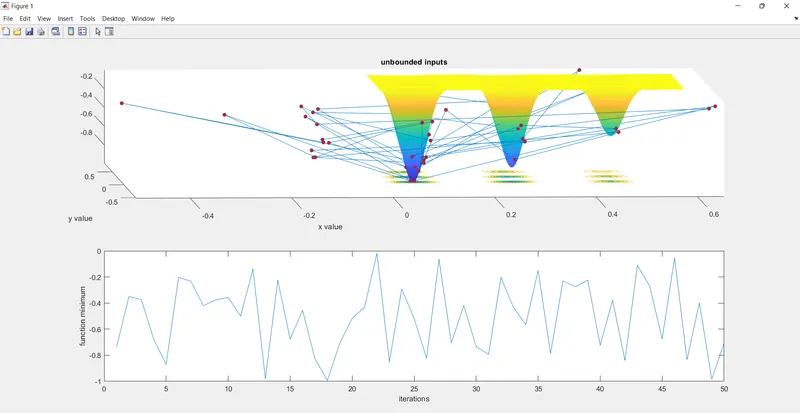
• statistical study with unbounded inputs, here the output we get varies within a disorder range.
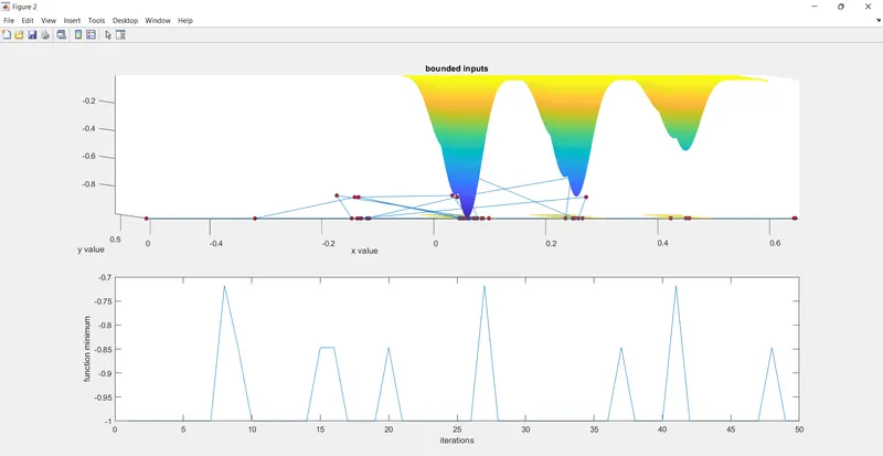
• statistical study with bounded inputs, here the output we get varies between the fixed desired range that we needed.
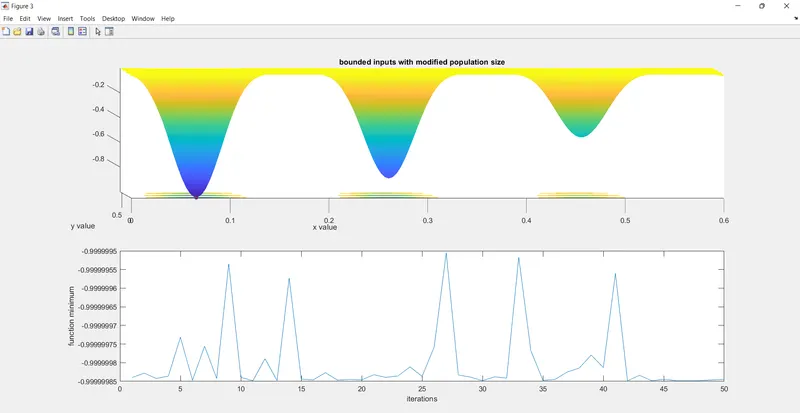
• By using the above 2 cases we get the optimal solution, but in order to get the more accurate solution, we increase the population size.
• That is our 3rd case bounded output with increased population.
• For each and every case we limited the no of iterations to 50.
• we need to increase the population size until only one point is obtained like as shown in the plot.

No errors during the compilation of the code.

References:

Matlab documentation for ga syntax.

used some google sites to know about the genetic algarithm.