Week 4.1 - Genetic Algorithm

Aim: To write a code in MATLAB to optimise the stalagmite function and find the global maxima of the function

Theory:

Understanding GA algorithm:

A genetic algorithm (GA) is a method for solving both constrained and unconstrained optimization problems based on a natural selection process that mimics biological evolution. The algorithm repeatedly modifies a population of individual solutions. At each step, the genetic algorithm randomly selects individuals from the current population and uses them as parents to produce the children for the next generation. Over successive generations, the population "evolves" toward an optimal solution.

You can apply the genetic algorithm to solve problems that are not well suited for standard optimization algorithms, including problems in which the objective function is discontinuous, nondifferentiable, stochastic, or highly nonlinear.

How does GA work?

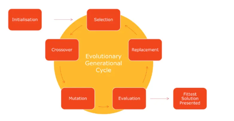
The Figure below shows the evolutionary cycle of a typical evolutionary algorithm. Each block represents an operation on a population of candidate solutions.

Initialization

The evolutionary process begins with initialization, wherein an initial population of candidate solutions is generated. There are many different methods of initializing populations, but with Genetic Algorithms the most popular method of initialization is simply to create a population of randomly initialized binary strings. Once the initial population has been created, the evolutionary generational cycle begins.

Selection

At each generational step, a pool of parents is chosen from the parent population based on the fitness values of each individual using a selection mechanism, such that the fittest individuals will have a greater probability of passing on genetic material to subsequent generations. This selected population (known as the “parent” population) then forms the basis for all subsequent optimizations during the generational step.

Variation

Once the parent population is fully populated via the selection process, a child population is created which will form the basis of the next generation. This child population is generated by variation operators, which are performed on individuals from the parent population. The most prominent such methods are crossover and mutation.

Crossover

Crossover takes pairs of parents from the parent population (usually random selection with replacement, such that the same parent can be selected multiple times to produce children). These parents then have some of their genetic information swapped between them. Crossover of two parent chromosomes is usually done in a single-point manner, where a single crossover point on both chromosomes is randomly selected and then all subsequent genetic information is swapped between individuals, as shown in Fig. 2:

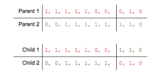
Figure(above): Single-point crossover of two parent GA chromosomes

Crossover is typically performed on randomly selected pairs of parents from the parent population until the new “child” population reaches the same size as the original parent population.

Mutation

While crossover simply swaps pre-existing information between pairs of candidate solutions, mutation in Evolutionary Algorithms is typically the standard method of introducing “new” genetic material into the population. Once the child population has been created via crossover, mutation in canonical Genetic Algorithms then occurs on all children in a “bit-flip” fashion by randomly changing codons on the chromosome between 0 and 1 (as shown in Fig. 3).

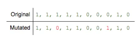
Figure(above): Bit-flip mutation of GA chromosome

Evaluation

Once the child population has been created, all children then need to be evaluated in order to assign a fitness value by which they can be judged against their peers. This fitness is used to sort/rank a population and to impose probabilities for both selection and replacement phases of the search process, such that the fittest members of the population have a higher probability of passing on genetic material.

Replacement

The final act of the generational step is to replace the old “N” population with the new “N+1” child population. While many methods exist, the most typical replacement method is Generational Replacement, wherein the entire previous generation is replaced with the newly generated child population.

Termination

A Genetic Algorithm will typically terminate after a predefined number of generations, or if some stopping criterion has been met (e.g. fitness is above some threshold, error rate is below some threshold, etc). The fittest solution in the population is then returned as the overall best solution.

GA syntax :

x = ga(fun,nvars,A,b,Aeq,beq,lb,ub,nonlcon,intcon,options) or

[x,fval] = ga(fun,nvars,A,b,Aeq,beq,lb,ub,nonlcon,intcon,options) where

fun - function handle to call the function.

nvars - number of variables

A ,b - Linear inequalities constraints

Aeq , beq - Linear equalities constraints

lb - lower bound

ub - upper bound

nonlcon - nonlinear constraints

intcon - integer constraint

options - optimization options

Equation:

`f(x,y) = f_(1x)f_(2x)f_(1y)f_(2y)`

`f_(1x) = [sin(5.1pix +0.5)]^6`

 `f_(1y) = [sin(5.1pix +0.5)]^6`

`f_(2x) = exp[-4log(2)(x-0.0667)^2/0.64]`

`f_(2y) = exp[-4log(2)(x-0.0667)^2/0.64]`

Procedure:

1.  The main Program starts with clear all, close all,clc
2. A search space is defined and it is converted into 2d with the help of meshgrid command.
3. A separate function code is written and the equation above is used(ga solver solves the equation to determine the max value)
4. Generally ga is used for find the minima in matlab, here in the code we have used the negative sign which indicates that the ga solver is actually calculating the max value.
5. The entire problem is analysed in 3 iteration.
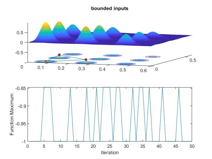
6. In the first time study or iteration from the plot we can observe that the ga solver is not picking the random inputs from the bounds of our population size mentioned in the code.Therefore in the second time study we have bounded the ga solver with minimum and max value of our space mentioned in the code.
7. The output of the second time study we can observe that the ga solver is picking 3 points to be the minimum value. To rectify this we can increased the population size.
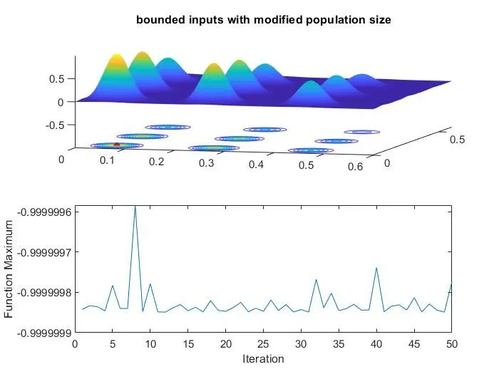
8. In the final time study we can observe that only one point as the max value , which is close to -1.
9. Therefore, we get the max value of our stalagmite function in the final time study.  

Stalagmite Function Code

function f = stalagmite_input_vector(input_vector)
x1 = input_vector(1);

y1 = input_vector(2);

f1_x = (sin((5.1*pi*x1) + 0.5)).^6;
f1_y = (sin((5.1*pi*y1) + 0.5)).^6;

f2_x = exp((-4*(log(2))*(x1-0.0667).^2)/0.64);
f2_y = exp((-4*(log(2))*(y1-0.0667).^2)/0.64);

f = -(f1_x*f2_x*f1_y*f2_y)

end

Stalagmite Main Code:

clear all
close all
clc

% Defining our search space

x = linspace(0,0.6,150);
y = linspace(0,0.6,150);
num_case = 50

% Creating 2D mesh
[xx, yy] = meshgrid(x,y)


% Evaluating a stalagmite Function

for i = 1:length(xx)
    for j = 1: length(yy)
        input_vector(1) = xx(i,j)
        input_vector(2) = yy(i,j)
        f(i,j) = stalagmite_input_vector(input_vector)
    end
end

tic
% Study 1 - Statistical Behaviour
for i = 1:num_case
    [inputs, fopt(i)] = ga(@stalagmite_input_vector, 2);
    xopt(i) = inputs(1);
    yopt(i) = inputs(2);
end
study1_time = toc

% Plotting 
figure(1)
subplot(2,1,1)
hold on
surfc(x, y, -f)
shading interp
plot3(xopt,yopt,-fopt,'marker','o','markersize',5,'markerfacecolor','r')
title('unbound inputs')
subplot(2,1,2)
plot(fopt)
xlabel('Iteration')
ylabel('Function Maximum')

tic
% Study 2 - With uper and lower bounds
for i = 1:num_case
     [inputs, fopt(i)] = ga(@stalagmite_input_vector, 2,[],[],[],[],[0;0],[0.6;0.6]);
     xopt(i) = inputs(1);
     yopt(i) = inputs(2);
end
study2_time = toc

% Plotting 
figure(2)
subplot(2,1,1)
hold on
surfc(x, y, -f)
shading interp
plot3(xopt,yopt,fopt,'marker','o','markersize',5,'markerfacecolor','r')
title('bounded inputs')
subplot(2,1,2)
plot(fopt)
xlabel('Iteration')
ylabel('Function Maximum')

tic
% Study 3 - Increasing ga iterations

options = optimoptions('ga');
options = optimoptions(options,'PopulationSize',170);


for i = 1:num_case
     [inputs, fopt(i)] = ga(@stalagmite_input_vector, 2,[],[],[],[],[0;0],[0.6;0.6],[],[],options);
     xopt(i) = inputs(1);
     yopt(i) = inputs(2);
end
study3_time = toc

% Plotting 
figure(3)
subplot(2,1,1)
hold on
surfc(x, y, -f)
shading interp
plot3(xopt,yopt,fopt,'marker','o','markersize',5,'markerfacecolor','r')
title('bounded inputs with modified population size')
subplot(2,1,2)
plot(fopt)
xlabel('Iteration')
ylabel('Function Maximum')

Output:

Study 1:

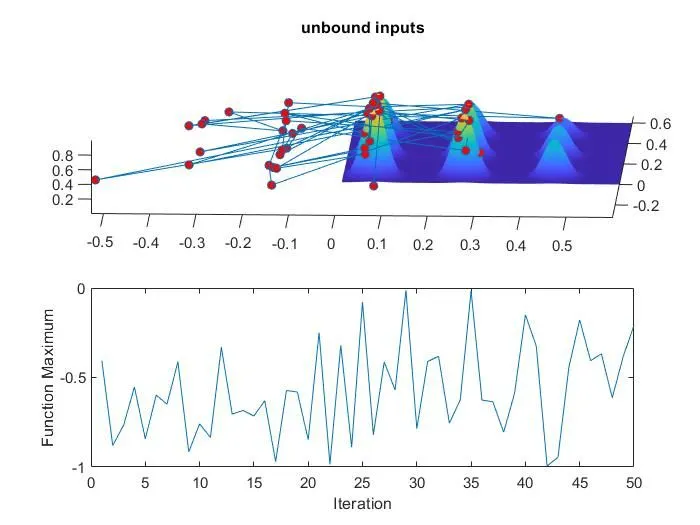
Study 2:

Study 3:

References:

https://www.pico.net/kb/how-does-a-genetic-algorithm-work/

https://in.mathworks.com/discovery/genetic-algorithm.html

https://skill-lync.com/knowledgebase/genetic-algorithm-explained