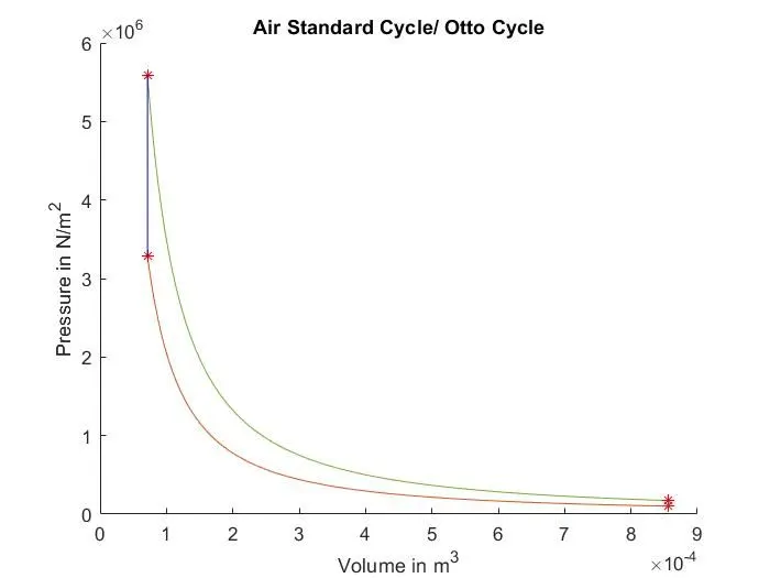
Plotting PV Diagram for an otto cycle using Matlab

Aim: To write a code that can solve an otto cycle and make plots for it.

Objective:

1. The code should create a PV diagram
2. Display the output of the thermal efficiency of the engine.

Theory:

The air-standard-Otto cycle is the idealized cycle for the spark-ignition internal combustion engines. This cycle is shown above on p-v diagrams. The Otto cycle 1-2-3-4 consists of following four process:

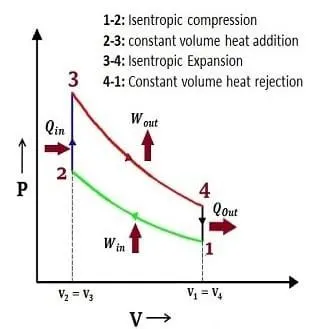
Process 1-2: Isentropic compression of air.
Process 2-3: Heat addition at constant volume.
Process 3-4: Isentropic expansion of air.
Process 4-1: Heat rejection at constant volume.

Governing Equation:

`V/(V(c)) = 1+1/2(r(c)-1)[R+1-costheta -(R^2 -sin^2theta)^(1/2)]`

The above formulae determines how volume inside an engine combustion chamber is going to change. This was derived purely from geometric relationships. This formulae is used here to code for a particular value of theta.

Thermal Efficiency of the engine:

`eta = 1 - 1/(cr)^(gamma-1)`

where

`eta =` Thermal Efficiency

cr = Compression Ratio

Other equation used to find the swept volume, clearance volume and state variables are given below

`Vs = pi/4 D^2L`

where : D - Bore Dia

L - Stroke length.

`Vc = (Vs)/(cr - 1)`

where: Vc - Clearance Volume

cr - compression ratio

Ideal Gas Equation:

`PV = nRT`

where : P - Pressure

V - Volume

T - Temperature

R - Ideal Gas Constant

Isentropic formulae:

`PV^gamma = constant`

Procedure:

1) The program starts with clear all, close all, clc

2) Inputs for the code are mentioned beforehand along with initial pressure and temperature state variables

3) The engine geometric parameters are also defined initially.

4) The swept volume and clearance volume are calculated by using the formulae above mentioned.

5) By using the isentropic formulae and ideal gas equation (where R=1, since the airfuel mixture is same and in the same environment) we can find the state variables across different stages.

6) A function code is written separately to store the different value of crank angle of rotation of compression and expansion occurs in different stoke. This function is then called to the main program accordingly.

7) The plots are then ploted accordingly with the help of plot command.

8) The thermal effiency is calculated by the formulae and the same is captured in the output window.

Function code:

function [V] = engine_kinematics(bore,stroke,con_rod,cr,start_crank,end_crank)

a = stroke/2;
R = con_rod/a;

v_s = pi/4 *bore^2*stroke;
v_c = v_s/(cr-1);

theta = linspace(start_crank,end_crank,100)

term1 = 0.5*(cr-1);
term2 = R+1-cosd(theta);
term3 = (R^2-sind(theta).^2).^0.5;

V = (1+term1*(term2-term3)).*v_c;
end

Final Code: To Plot PV Diagram :

clear all 
close all
clc


% Inputs
gamma = 1.4;
t3 = 2300


%State Variables
p1 = 101325
t1 = 500

%Engine geometric parameters

bore = 0.1;
stroke = 0.1;
con_rod = 0.15;
cr = 12;

% calculating the swept volume and clearance volume
v_swept = (pi/4)*bore^2*stroke;
v_clearance = v_swept/(cr-1);
v1 = v_swept+v_clearance;
v2 = v_clearance;

% state varaibles at state point 2
% p2v2^gamma = p1v1^gamma 
% p2 = p1*(v1/v2)^gamma = p1*cr^gamma
 p2 = p1*cr^gamma
 
 %p1v1/t1 = p2v2/t2 | t2 = p2*v2*t1/(p1*v1)
 t2 = p2*v2*t1/(p1*v1)
 
 constant_c = p1*v1^gamma;
  V_compression = engine_kinematics(bore,stroke,con_rod,cr,180,0);
 
  P_compression = constant_c./V_compression.^gamma;
  
  
 %state variables at state point 3
 v3 = v2
 
 %p3v3/t3 = p2v2/t2 | p3 = p2*t3/t2
 
 p3 = p2*t3/t2
 
 constant_c = p3*v3^gamma;
  V_expansion = engine_kinematics(bore,stroke,con_rod,cr,0,180);
 
  P_expansion = constant_c./V_expansion.^gamma;
  
 
 % state varaibles at stae point 4
  v4 = v1;
  
  % p3v3^gamma = p4v4^gamma | p4 = p3*(v3/v4)^gamma
  
  p4 = p3*(v3/v4)^gamma
  
  % Thermal Efficiency of the engine
  
  Thermal_efficiency = 1-(1/cr^(gamma-1))
  
  figure(1)
  hold on
  plot(v1,p1,'*', 'color', 'r')
  plot( V_compression , P_compression)
  plot(v2,p2,'*', 'color', 'r')
  plot(v3,p3,'*', 'color', 'r')
  plot( V_expansion , P_expansion)
  plot(v4,p4,'*', 'color', 'r')
  plot([v2 v3],[p2 p3],'color','b')
  plot([v4 v1],[p1 p4])
  ylabel('Pressure in N/m^2')
  xlabel('Volume in m^3')
  title('Air Standard Cycle/ Otto Cycle')

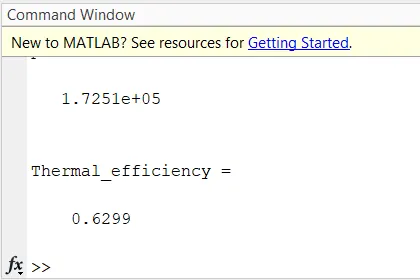
Thermal Efficiency output : 62.99%

Error1:

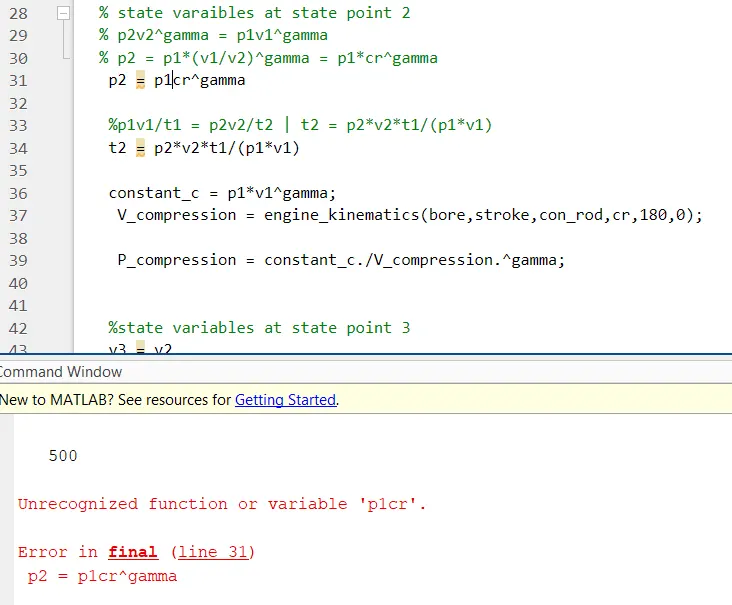
Solution : missing multiplication operator. Corrected by p2 = p1*cr^gamma.

Error2

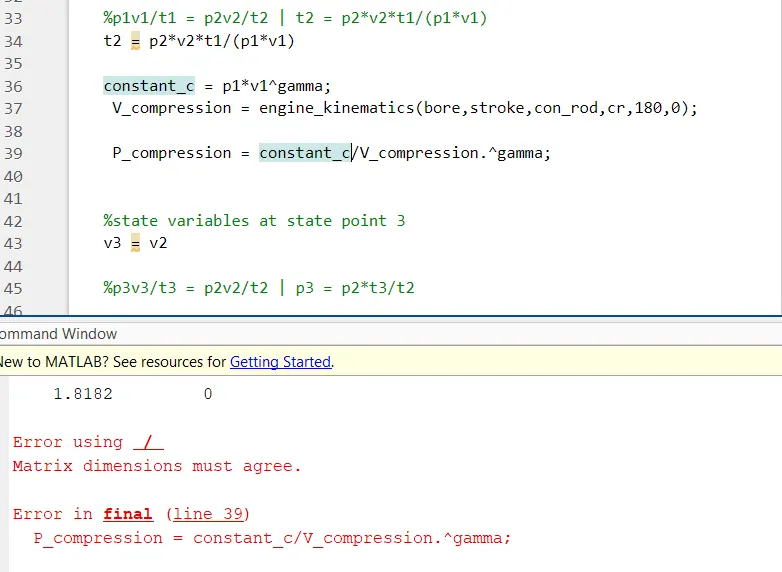
Solution : Missing dot operator . Corrected expression: P_compression = constant_c./V_compression.^gamma

The PV Diagram Plot: