Week 4.1 - Genetic Algorithm
Aim: To generate a MATLAB code to perform optimisation process
Objectives:
Basically, Genetic algorithm is used to calculate minimum value of the optimisation problem. But our aim is to calculate the maximum values for the given problem, to get maximum values we are inverting plot by applying “-f ”.
Optimisation:
Optimisation is a decision making process, it helps to find the best results under a set of prioritized criteria or constraints. It is a procedure which is executed iteratively by comparing various solutions till an optimum or a satisfactory solution is found.
These include maximizing factors such as productivity, strength, reliability, efficiency, utilization, etc
Example:
Let’s take, you are designing a simply supported beam to withstand the load of 1-tonne, in this case you need to consider the following parameters: Length, breadth, width, factor of safety, weight and stress induced. Here optimization helps to find the best value for length, breadth and width of the beam in such a way that the factor of safety, material consumed and stress induced are within the limit.
Different techniques available to perform optimisation:
- Deterministic Method
- Stochastic Method
Deterministic Method:
They use specific rules for moving one solution to another. In this technique, the output of the model is fully determined by the parameter values and the initial conditions.
Example:
Stress analysis of the component, this is a deterministic approach since the output results (stress values) fully depend on the initial conditions (loading condition) and the parameter values (force acting on the component and material properties).
Stochastic Method:
These are gaining popularity due to certain properties which deterministic algorithms do not possess. Stochastic models possess some inherent randomness, it is a probabilistic approach.
Example:
Varying the water paths from the mountain can vary the regional weather conditions, but the weather condition is not fully dependent on the water paths, hence there will be many statistical predictions to get the predictive model, since the weather condition depends on various factors such as solar distance, latitudinal location, air pressure, etc. Hence it is a predictive model.
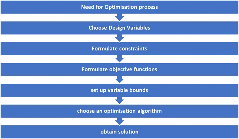
Step by step procedure for the optimisation process:
Terms frequently used in this process:4
Variables:
The parameters which you have to vary during the optimisation process are known as variables.
Example: Design dimensions can be varied to get the minimum stress.
Constraints:
During the optimisation process, your output should not go beyond the certain limits, those are known as constraints.
Example: You can reduce the material used in such a way that the stress should not go beyond the ultimate stress of the material.
Objective function:
Objective function is as simple as a mathematical formula, which can be a predicted mathematical model that includes all the variables as input. Example: z=f(x,y) here the output(z) depends on the input variable(x&y).
Variable bounds:
The variable bounds are the range of the input variables, that will be varied for every iteration to provide an optimised result.
Example: The design variable (thickness) can be varied in the range between (5-7) mm, to get the minimum stress.
Genetic Algorithm:
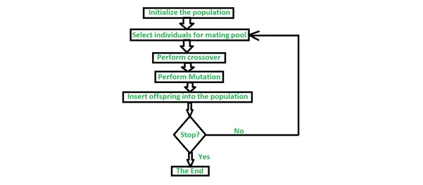
As shown above in the flowchart, we need to choose an optimisation algorithm to perform the optimisation process. Genetic algorithm is one of the optimisation processes. Genetic Algorithm (GA) is a search-based optimization technique based on the principles of Genetics and Natural Selection. It is frequently used to find optimal or near-optimal solutions. It is frequently used to solve optimization problems, in research, and in machine learning.
step by step process for optimisation process
GA flow chart
Information about the optimization process, returned as a structure with these fields:
Problem type — Problem type, one of:
- 'Unconstrained'
- 'Bound constraints'
- 'Linear constraints'
- 'Nonlinear constr'
- 'Integer constraints'
GA SYNTAX in MATLAB:
- x = ga(fun,nvars)
finds a local unconstrained minimum, x, to the objective function, fun.nvars is the dimension (number of design variables) of fun.
- x = ga(fun,nvars,A,b)
finds a local minimum x to fun, subject to the linear inequalities A*x ≤ b. ga evaluates the matrix product A*x as if x is transposed (A*x').
- x = ga(fun,nvars,A,b,Aeq,beq)
finds a local minimum x to fun, subject to the linear equalities Aeq*x = beq and A*x ≤ b. (Set A=[] and b=[] if no linear inequalities exist.) ga evaluates the matrix product Aeq*x as if x is transposed (Aeq*x').
- x = ga(fun,nvars,A,b,Aeq,beq,lb,ub) defines a set of lower and upper bounds on the design variables, so that a solution is found in the range lb ≤ x ≤ ub. (Set Aeq=[] and beq=[] if no linear equalities exist.)
- x = ga(fun,nvars,A,b,Aeq,beq,lb,ub,nonlcon) subjects the minimization to the constraints defined in nonlcon. The function nonlcon accepts x and returns vectors C and Ceq, representing the nonlinear inequalities and equalities respectively. ga minimizes the fun such that C(x) ≤ 0 and Ceq(x) = 0. (Set lb=[] and ub=[] if no bounds exist.)
- x = ga(fun,nvars,A,b,Aeq,beq,lb,ub,nonlcon,options) minimizes with the default optimization parameters replaced by values in options. (Set nonlcon= [] if no nonlinear constraints exist.) Create options using optimoptions.
- x = ga(fun,nvars,A,b,[],[],lb,ub,nonlcon,IntCon) or
x = ga(fun,nvars,A,b,[],[],lb,ub,nonlcon,IntCon,options) requires that the variables listed in IntCon take integer values.
- x = ga(problem) finds the minimum for problem, where problem is a structure.
- [x,fval] = ga(___),
for any previous input arguments, also returns fval, the value of the fitness function at x.
- [x,fval,exitflag,output] = ga(___) also returns exitflag, an integer identifying the reason the algorithm terminated, and output, a structure that contains output from each generation and other information about the performance of the algorithm.
- [x,fval,exitflag,output,population,scores] = ga(___) also returns a matrix population, whose rows are the final population, and a vector scores, the scores of the final
MATLAB code explanation:
- Defining x, y values from 0 to 150 with a difference of 0.6
x=linspace (0,0.6,150);
y=linspace (0,0.6,150);
- Genetic algorithm is runs for 50 times
num_case=50;
- Generating 2D Array
[xx,yy]=meshgrid(x,y);
- Evaluating stalagmite function
for i=1:length(xx)
for j=1:length(yy)
input_vector(1)=xx(i,j);
input_vector(2)=yy(i,j);
f(i,j)=stalgamite(input_vector);
end
end
- Creating a three-dimensional surface
figure(1)
surfc(xx,yy,-f)
shading interp % for shading surface more smoother
xlabel('x value');
ylabel('y label');
title('stalgamite function');
- Case1:
GA is running for unbounded input values
tic % for calculating optimisation time
for i=num_case
[inputs,f_opt(i)]=ga(@stalgamite,2);
x_opt(i)=inputs(1);
y_opt(i)=inputs(2);
end
study1_time=toc;
plotting on a plot
figure(2)
subplot(2,1,1)
hold on
surfc(x,y,-f)
title('unbounded inputs')
xlabel('x value')
ylabel('y value')
zlabel('function values')
shading interp
hold on
plot3(x_opt,y_opt,-f_opt,'marker','o','markersize',5,'MarkerFaceColor','r');
subplot(2,1,2)
plot(-f_opt)
xlabel('iterations')
ylabel('function maximum')
zlabel('function values')
- Case2:
optimisation process between the lower and upper bounds
tic % for time counting
for i=num_case
[inputs,f_opt(i)]=ga(@stalgamite,2,[],[],[],[],[0;0],[0.6;0.6]);
% optimum values are calculating between 0 to 0.6
x_opt(i)=inputs(1);
y_opt(i)=inputs(2);
end
study2_time=toc
plotting
figure(3)
subplot(2,1,1)
surfc(x,y,-f)
shading interp
title('Bounded inputs')
xlabel('x values')
ylabel('y values')
hold on
plot3(x_opt,y_opt,-f_opt,'marker','o','markersize',5,'MarkerFaceColor','r');
subplot(2,1,2)
plot(-f_opt)
xlabel('iteration')
ylabel('function maximum')
Case3:
Increasing the population size with lower and upper bounds
tic
for i=1:num_case
[inputs,f_opt(i)]= ga(@stalgamite,2,[],[],[],[],[0;0],[0.6;0.6],[],[],options);
x_opt3(i)=inputs(1);
y_opt3(i)=inputs(2);
end
study3_time=toc % gives the time taken for the study
plotting
figure(4)
subplot(2,1,1)
surfc(x,y,-f) % create a surface to visualise in 3D
shading interp
title('bounded inputs with higher population size')
xlabel('x axis')
ylabel('y axis')
zlabel('function values')
hold on
plot3(x_opt3,y_opt3,-f_opt,'Marker','o','MarkerSize',5,'MarkerFaceColor','r');
subplot(2,1,2)
plot(-f_opt)
xlabel('x axis-iterations')
ylabel('y axis-maxvalue')
- To create optimisation options
options=optimoptions(@ga)
option=optimoptions(@ga,'PopulationSize',500)
% Increasing the population size
STALGAMITE FUNCTION:
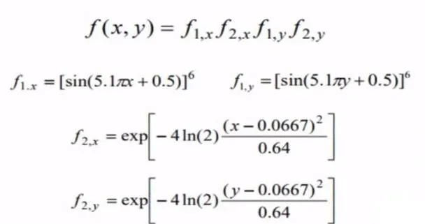
function input = stalgamite(input_vector)
x=input_vector(1);
y=input_vector(2);
f1x=[sin((5.1*pi*x+0.5))].^6;
f2y=[sin((5.1*pi*y+0.5))].^6;
f3x=exp(-4*log(2)*((x-0.667).^2/0.64));
f4y=exp(-4*log(2)*((y-0.667).^2/0.64));
f=(f1x*f3x*f2y*f4y);
input=-f
% -ve sign is used as the genetic algoritham returns the global maxima but we need the global maxima
end
clear all
close all
clc
x=linspace(0,0.6,150);
y=linspace(0,0.6,150);
% number of iterations
num_case=50;
[xx,yy]=meshgrid(x,y);
% evaluating values of stalgamite function
for i=1:length(xx)
    for j=1:length(yy)
        input_vector(1)=xx(i,j);
        input_vector(2)=yy(i,j);
        f(i,j)=stalgamite(input_vector);
    end
end
% creates a three dimensional surface
figure(1)
surfc(xx,yy,-f)
shading interp  % for shading surface more smoother
xlabel('x value');
ylabel('y label');
title('stalgamite function');

% case study1, unbounded inputs
tic     % for calculating optimisation time
for i=num_case
    [inputs,f_opt(i)]=ga(@stalgamite,2);
    x_opt(i)=inputs(1);
    y_opt(i)=inputs(2);
end
study1_time=toc
figure(2)
subplot(2,1,1)
hold on
surfc(x,y,-f)
title('unbounded inputs')
xlabel('x value')
ylabel('y value')
zlabel('function values')
shading interp
hold on
plot3(x_opt,y_opt,-f_opt,'marker','o','markersize',5,'MarkerFaceColor','r');
% optimum values are calculating between 0 to 0.6
subplot(2,1,2)
plot(-f_opt)
xlabel('iterations')
ylabel('function maximum')
zlabel('function values')
% for case 2 upper and lower bounds
tic
for i=num_case
    [inputs,f_opt(i)]=ga(@stalgamite,2,[],[],[],[],[0;0],[0.6;0.6]);
    x_opt(i)=inputs(1);
    y_opt(i)=inputs(2);
end
study2_time=toc
figure(3)
subplot(2,1,1)
surfc(x,y,-f)
shading interp
title('Bounded inputs')
xlabel('x values')
ylabel('y values')
hold on
plot3(x_opt,y_opt,-f_opt,'marker','o','markersize',5,'MarkerFaceColor','r');
subplot(2,1,2)
plot(-f_opt)
xlabel('iteration')
ylabel('function maximum')

% case study3 increasing the population size with upper bound lower bound
% by doing so we are increasing the probability
%to converge at global maxima

options=optimoptions(@ga)
option=optimoptions(@ga,'PopulationSize',500)    % increasing the population size
tic
for i=1:num_case
    [inputs,f_opt(i)]= ga(@stalgamite,2,[],[],[],[],[0;0],[0.6;0.6],[],[],options);
    x_opt3(i)=inputs(1);
    y_opt3(i)=inputs(2);
end
study3_time=toc  % gives the time taken for the study
figure(4)
subplot(2,1,1)
surfc(x,y,-f)   % create a surface to visualise in 3D
shading interp
title('bounded inputs with higher population size')
xlabel('x axis')
ylabel('y axis')
zlabel('function values')
hold on
plot3(x_opt3,y_opt3,-f_opt,'Marker','o','MarkerSize',5,'MarkerFaceColor','r');
subplot(2,1,2)
plot(-f_opt)
xlabel('x axis-iterations')
ylabel('y axis-maxvalue')
RESULTS:
In case we get better result.the optimum value is 0.68