Week 3 - Solving second order ODEs

SIMPLE PENDULUM:

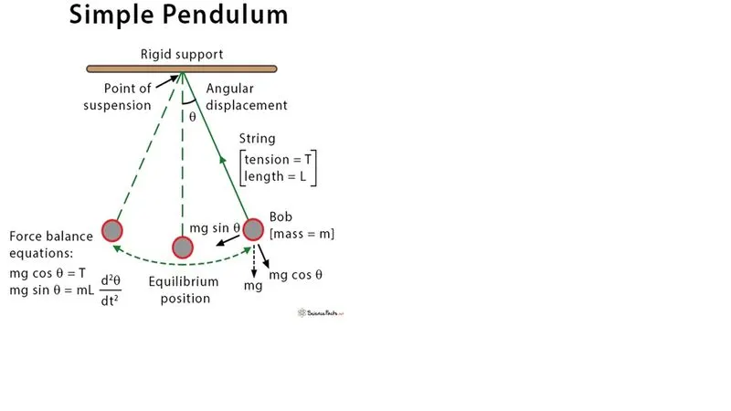
• • • A pendulum is a body suspended from a fixed support so that it swings freely back and forth under the influence of gravity.
    • When a pendulum is displaced sideways from its resting, equilibrium position, it is subject to a restoring force due to gravity that will accelerate it back toward the equilibrium position.
    • When released, the restoring force acting on the pendulum's mass causes it to oscillate about the equilibrium position, swinging it back and forth.
    • The mathematics of pendulums are in general quite complicated. Simplifying assumptions can be made, which in the case of a simple pendulum allow the equations of motion to be solved analytically for small-angle oscillations.
    • The differential equation which represents the motion of a simple pendulum is {\displaystyle {\frac {d^{2}\theta }{dt^{2}}}+{\frac {g}{\ell }}\sin \theta =0}
    • τ=Iα⇒ −mg sinθ L=mL²d²θ/dt²
    • and rearranged as d²θ/dt² + gLsinθ =0

    b=0.05;
    g=9.81;
    l=1;
    m=0.1;

  • 

    clear all
    close all
    clc
    % inputs
    b=0.05;
    g=9.81;
    l=1;
    m=0.1;
    % initial condition
    theta_0=[0 3];
    % time points
    t_span=linspace(0,20,200);
    % solving ODE
    [t,results]= ode45(@(t,theta) ode_func(t,theta,b,g,l,m),t_span,theta_0);
    figure(1)
    plot(t,results(:,1))
    hold on
    plot(t,results(:,2))
    xlabel('TIME')
    ylabel('PLOT')
    legend('dispacement','velocity')
    
    ct=1;
    results_loop=results(:,1);
    for i=1:length(results(:,1))
        x0=0;
        y0=0;
        loop=results_loop(i);
        x1=l*sin(loop);
        y1=-l*cos(loop);
        figure(2)
        plot([-1 1],[0 0],'linewidth',3)
        hold on
        plot([x0 x1],[y0 y1],'linewidth',1,'Color','b')
        axis([-1.5 1.5 -1.5 1.5])
        plot (x1,y1,'o','MarkerSize',20,'MarkerFaceColor','r')
        hold off
        M(ct)=getframe(gcf)
        ct=ct+1;
    end
    % making the video file
    movie(M)
    videofile=VideoWriter('solving simple_pendulum.avi')
    open(videofile)
    writeVideo(videofile,M)
    close(videofile)
    

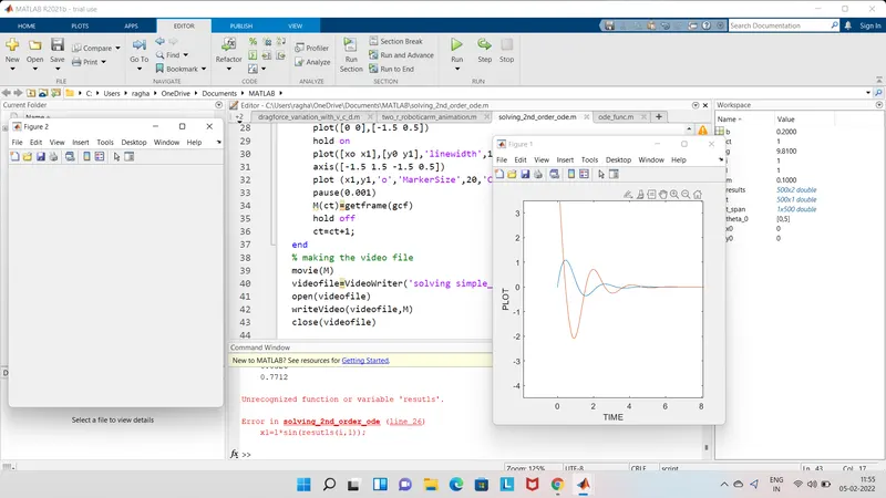
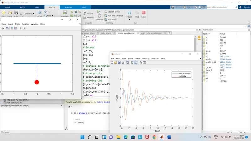
    Execution images :

  • 

  • 

https://drive.google.com/file/d/1ep6s0_4nOLdie2g51csxRbg_pg7UcV-C/view?usp=sharing