Week 4.1 - Genetic Algorithm
AIM: 1) To write a code in Matlab, to optimize the stalagmite function and find the Global maxima of the function.
2) To explain the concept of genetic algorithm.
3) To plot graph between F maximum versus no. of iterations.
CONCEPT OF GENETIC ALGORITHM:
The concept of genetic algorithm is based upon the survival of the fittest. like, the principle is based upon the biological evolution. Moving to procedure of Genetic algorithm, it starts with random population of points and generates random population of points called individuals at each iteration called generation of algorithm.
Genetics algorithm uses three operators and these are :
1)SELECTION
2)CROSSOVER and
3) MUTATION
Selection operator just identifies the parents from the population whereas crossover operator applies to two parents that are randomly selected and are matched in order to produce childrens. Also, the mutation operator is applied to find out the diversity in population .
These operations are performed during each generation or iteration and algorithm stops when population can no longer be improved or the maximum number of iterations has been reached.
Two functions in the matlab are used based on GA:
1)ga- for single objective optimization problem
2) gamultiobj- for multi objective optimization problem
POINTS TO PONDER FOR GENETIC ALGORITHM:
1) In genetic algorithm, the functions are highly non-linear, non-differential and discontinuous. However, the design variables can be continous or discrete or combination of both.
2) The GA method requires the values of the objective function or constraint function but not the derivatives of the same to reach the optimum value. Also, this method can converge to global optimum.
SYNTAX FOR GENETIC ALGORITHM :
- X= ga(fun,nvars)
It finds a local unconstrained minimum ‘x’, to the objective function(fun). nvars is the dimension(number of designed variables) of function(fun).
- X=ga(fun,nvars,A,b)
It finds a local minimum and subjected to linear inequalities A*xb.
- X=ga(fun, navrs, A, b, Aeq, beq)
It finds local minimum which is subjected to linear inequalities Aeq*x=beq and A*x≤b.
- X=ga(fun, navrs, A, b, Aeq, beq, lb, ub)
It defines a set of lower and upper bounds in the design variables x, so that a solution is found in the range ‘lb≤x≤ub’.
- X=ga(fun, navrs, A, b, Aeq, beq, lb, ub, nonlcon)
It subjects the minimization to the constraints defined in nonlcon. The function nonlcon accepts x and returns vectors C and Ceq, representing the nonlinear inequalities and equalities respectively.
- X=ga(fun, navrs, A, b, Aeq, beq, lb, ub, nonlcon, options)
It minimizes with the default optimization parameters replaced by values in ‘options’.
- X=ga(fun, navrs, A, b, Aeq, beq, lb, ub, nonlcon, Intcon)
It takes integer values listed in ‘intcon’.
- X=ga(problem)
Finds the minimum for ‘problem’, a structured described in ‘problem’.
- [x ,fval]=ga(_____)
For any input arguments, also returns ‘fval’, the value of the fitness function at ‘x’.
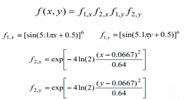
THE STALAGMITE FUNCTION THAT HAS BEEN OPTIMISED USING GA IS SHOWN BELOW:
THE CODE FOR THE ABOVE PROGRAM IN MATLAB IS SHOWN BELOW:
function f= stalagmite(input_vector)
x=input_vector(1);
y=input_vector(2);

f1=(sin(5.1*pi*x+0.5))^6;
f2=(sin(5.1*pi*y+0.5))^6;
f3=exp(-4*log(2)*(x-0.0667)^2/0.64);
f4=exp(-4*log(2)*(y-0.0667)^2/0.64);
f=-(f1*f2*f3*f4);


end
1ST ITERATION:
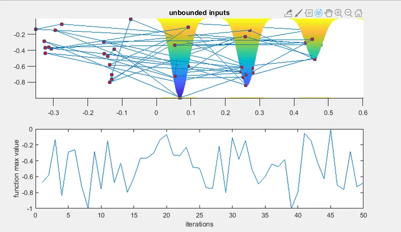
1)Moving on to the first iterations , it is unbounded, that is, without any limits and the program for the following is as given below:
%This is the first iteration and is unbounded that is without any limits

clear all
close all
clc


%creating a reigon
x=linspace(0,0.6,150);
y=linspace(0,0.6,150);


% creating a Meshgrid
[xx,yy]=meshgrid(x,y);


% CREATING SURFACE PLOT FOR STALAGMITE FUNCTION
for i=1:length(xx)
    for j=1:length(yy)
        input_vector(1)=xx(i,j);
        input_vector(2)=yy(i,j);
        f(i,j)=stalagmite(input_vector);
    end
end

num_cases=50; %GA runs for 50 iterations
tic %study time count starts

for i=1:num_cases
    [inputs,f_opt(i)]=ga(@stalagmite,2);% ga function is used to run the stalagmite data
    x_opt(i)=inputs(1);
    y_opt(i)=inputs(2);
    opt_f(i)=f_opt(i); %ga gives us minima value. Inverse is taken for maxima value

end

study1_time=toc %study time count end

%plotting the graph

subplot(2,1,1)
hold on
surfc(xx,yy,f);

shading interp
plot3(x_opt, y_opt,opt_f,'marker','o','markersize',5,'markerfacecolor','r')
title('unbounded inputs')
subplot(2,1,2)

plot(opt_f)
xlabel('iterations')
ylabel('function max value')
Results obtained from the first unbounded iteration are shown below:
2ND ITERATIONS:
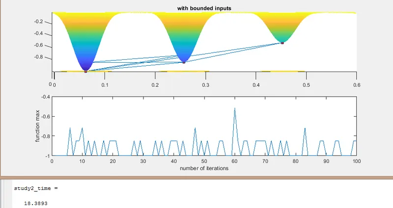
In this 2nd iteration, number of cases has been extended to 100 in the command num_cases=100 and is bounded with upper bound by 0.6.
% program for 2nd iteration

clear all
close all
clc

x=linspace(0,0.6,150); %x input values
y=linspace(0,0.6,150);  %y input values


%creating a meshgrid
[xx,yy]=meshgrid(x,y);

for i=1:length(xx)
    for j=1:length(yy)
        input_vector(1)=xx(i,j);
        input_vector(2)=yy(i,j);
        f(i,j)=stalagmite(input_vector);
    end
end

num_cases=100; %ga runs for 100 iterations
tic % study time start
for i=1:num_cases;
    %objecctive function is stalagmite and the number of variabes are 2.
    % A,B,Aeq,Beq=[], as there is no linear inequalities and equalities
    % constraints in this function
    % lower boundry variable x and y in this  ga  is set as [0,0]
    %upper boundry of variables x and y in this ga is set as [0.6, 0.6]
    [inputs,f_opt(i)]=ga(@stalagmite,2,[],[],[],[],[0,0],[0.6,0.6]);
    x_opt(i)=inputs(1);
    y_opt(i)=inputs(2);
    opt_f(i)=f_opt(i);
end
study2_time=toc %study time ends

subplot(2,1,1)
hold on
surfc(xx,yy,f) %genrating the stalagmite function
shading interp

plot3(x_opt,y_opt,f_opt,'marker','o','markersize',5,'markerfacecolor','r')
title('with bounded inputs')
subplot(2,1,2)

plot(opt_f) % plotting opt_f value for every iteration
xlabel('number of iterations')
ylabel('function max')
RESULTS FROM THE ABOVE CODING ARE SHOWN BELOW:
3rd ITERATION:
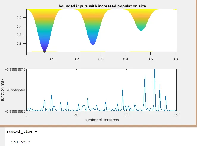
In this iteration, i have increased the population size with bounded inputs.
% program for 3rd iteration

clear all
close all
clc

x=linspace(0,0.6,150); %x input values
y=linspace(0,0.6,150);  %y input values


%creating a meshgrid
[xx,yy]=meshgrid(x,y);

for i=1:length(xx)
    for j=1:length(yy)
        input_vector(1)=xx(i,j);
        input_vector(2)=yy(i,j);
        f(i,j)=stalagmite(input_vector);
    end
end

num_cases=150; %ga runs for 150 iterations
options=optimoptions('ga');
options=optimoptions(options,'PopulationSize',450);
tic % study time start
for i=1:num_cases;
    %objecctive function is stalagmite and the number of variabes are 2.
    % A,B,Aeq,Beq=[], as there is no linear inequalities and equalities
    % constraints in this function
    % lower boundry variable x and y in this  ga  is set as [0,0]
    %upper boundry of variables x and y in this ga is set as [0.6, 0.6]
    [inputs,f_opt(i)]=ga(@stalagmite,2,[],[],[],[],[0,0],[0.6,0.6],[],options);
    x_opt(i)=inputs(1);
    y_opt(i)=inputs(2);
    opt_f(i)=f_opt(i);
end
study2_time=toc %study time ends

subplot(2,1,1)
hold on
surfc(xx,yy,f) %genrating the stalagmite function
shading interp

plot3(x_opt,y_opt,f_opt,'marker','o','markersize',5,'markerfacecolor','r')
title(' bounded inputs with increased population size')
subplot(2,1,2)

plot(opt_f) % plotting opt_f value for every iteration
xlabel('number of iterations')
ylabel('function max')
The results for the above code are shown below:
ERRORS FACED WHILE PROGRAMMING:
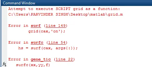
Here above, i did mistake in for loop command and it was continously displayed in the 'surfc' command . So i corrected my mistake, as it was a typo and then the error was omitted.
References:
1) youtube/YARPIZ
2)engineer's guide to Matlab by Edward.B Magrab
3) mathswork.com/matlab