Project 2 - Rankine cycle Simulator
PROJECT AIM: RANKINE CYCLE SIMULATOR
OBJECTIVES TO ACCOMPLISH:-1) Calculate the state points of the rankine cycle based on user inputs.
2) Plot the corresponding T-s and h-s plots for the given set of inputs.
BASIC CONCEPTS AND DEFINITIONS:-
1) Isentropic process:- It is a thermodynamic process that is both adiabatic and reversible. Also, work transfer of the system is frictionless and there is no net heat transfer.
2) Adiabatic process:- Process which doesn't required transfer of heat and mass between the system and its surroundings.
3) RANKINE CYCLE:- It is an idealized thermodynamic cycle in which mechanical work is extracted from the fluid as it moves between heat source and heat sink.
4) Dryness fraction:- It is the ratio of mass of actual dry steam to the mass of steam containing and it is usually expressed by X.
5) Specific steam consumption:- It is defined as the steam consumed by a locomotives's cylinders per unit output of power. It is typically measured in kg/kJ.
ALL ABOUT RANKINE CYCLE
Rankine cycle is an ideal cycle for vapor power cycle and power plants based on such cycle generate electrical power by using fuels like coal, oil or natural gas. The diagram of rankine cycle is shown above. Moving to the working of rankine cycle, fuel burnt in the boiler heats the water to generate superheated steam. This steam is used to run the turbine which powers can power the generator.After the steam leaves the turbine, it is cooled to its liquid state in the condenser by transferring heat to the cooling water system.The liquid is pressurized by pump prior to going back to the boiler.
1-2 Isentropic expansion in the turbine:- High pressure liquid enters the boiler and is heated to the saturation point. Further addition of energy causes evaporation of the liquid until it is fully converted to saturated steam.
2-3:- Isentropic Expansion in the turbine:- The vapor is expanded in the turbine thus producing the work which may be converted to electricity.
3-4:- Isobaric Heat rejection:-The vapor liquid mixture leaving the turbine is condensed at low pressure.
4-1:-Isentropic compression :- The pressure of the condensate is raised in the feed pump. Because of the low specific volume of liquid, pump work is relatively small.
MAIN PROGRAM:-
clear
close all
clc

fprintf('     SIMULATOR OF RANKINE CYCLE \n') %\n is used for new line character
fprintf('1-2 ISENTROPIC EXPANSION IN TURBINE \n')
fprintf('2-3 CONSTANT PRESSURE HEAT REJECTION BY THE CONDENDER \n')
fprintf('3-4 ISENTROPIC COMPRESSION IN THE PUMP \n')
fprintf('4-1 CONSTANT PRESSURE HEAT ADDITION BY THE BOILER \n')

% fprintf command is used to display the statements in the command window.


%INPUTS command is used to undertake values from the different characters
P1=input('Enter the pressure at the turbine inlet(in bar):');
T1=input('Enter the temperature at the turbine inlet(in degree celcius):');
P2=input('Enter the pressure at the condenser(in bar):');
disp('  RESULTS') %used for diplaying results in the command window


% EXTRACTING cp and cv values from the xsteam for vapors
high_cpV=XSteam('cpV_p',P1);
low_cpV=XSteam('cpV_p',P2);
high_cvV=XSteam('cvV_p',P1);
low_cvV=XSteam('cvV_p',P2);


%EXTRACTING cp and cv VALUES FROM THE XSteam FOR LIQUIDS
high_cpL=XSteam('cpL_p',P1);
low_cpL=XSteam('cpL_p',P2);
high_cvL=XSteam('cvL_p',P1);
low_cvL=XSteam('cvL_p',P2);


%EXTRACTING USABLE PARAMETERS FROM THE XSteam specifically for high
%pressure

T1s=XSteam('Tsat_p',P1);
S1g=XSteam('sV_p',P1);
S1f=XSteam('SL_p',P1);
S1fg=S1g-S1f;
H1f=XSteam('hL_p',P1);
H1g=XSteam('hV_p',P1);
H1fg=H1g-H1f;


%Extracting usable parameters from the xsteam for low pressure

S2g=XSteam('sV_p',P2);
S2f=XSteam('SL_p',P2);
S2fg=S2g-S2f;
T2s=XSteam('Tsat_p',P2);
H2f=XSteam('hL_p',P2);
H2g=XSteam('hV_p',P2);
H2fg=H2g-H2f;


%% STATE POINT 1
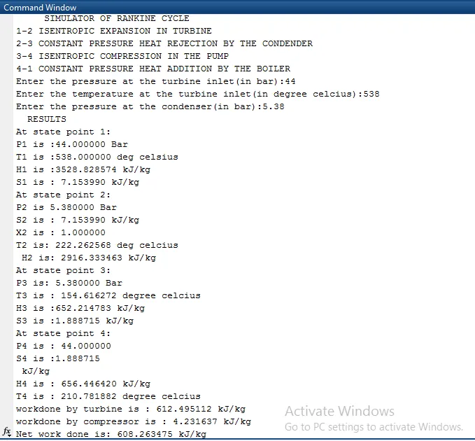
disp('At state point 1:')
fprintf('P1 is :%f Bar \n',P1)
fprintf('T1 is :%f deg celsius \n',T1)

H1=XSteam('h_pt',P1,T1);
fprintf('H1 is :%f kJ/kg \n',H1)

S1=XSteam('s_pt',P1,T1);
fprintf('S1 is : %f kJ/kg \n',S1)


%% STATE POINT 2
disp('At state point 2:')
fprintf('P2 is %f Bar \n',P2)

S2=S1;
fprintf('S2 is : %f kJ/kg \n',S2)

%Predicting location of point 2 in T-s

if (S2<=S2g)
    X2=(S2-S2f)/(S2fg)   ;   % DRYNESS FRACTION CALCULATION
else
    X2=1;

end
fprintf('X2 is : %f \n',X2)

% calculating T2 for superheated reigon
if (X2<1)
    T2=T2s;
else

T2=(T2s+273.15)*exp((S2-S2g)/low_cpV);
T2=T2-273.15;

end
fprintf('T2 is: %f deg celcius \n',T2)

if(X2<1)
    H2=H2f+X2*H2fg;
else
    H2=H2g+low_cpV*(T2-T2s);
end
fprintf(' H2 is: %f kJ/kg \n',H2)


%% state point 3
%ASSUMED NO SUBCOOOLING IN CONDENSER

disp('At state point 3:')

P3=P2;
fprintf('P3 is: %f Bar \n',P3)

V3=XSteam('vL_p',P3);

T3=T2s;  %NO SUBCOOLING ASSUMED
fprintf('T3 is : %f degree celcius \n',T3)

H3=H2f;
fprintf('H3 is :%f kJ/kg \n',H3);

S3=S2f;
fprintf('S3 is :%f kJ/kg \n',S3)


%% state point 4
disp('At state point 4:')

P4=P1;
fprintf('P4 is : %f \n', P4)

S4=S3;
fprintf('S4 is :%f \n kJ/kg \n',S4)

Wp=V3*(P4-P3)*100;
H4=Wp+H3;
fprintf('H4 is : %f kJ/kg \n',H4)


% TO CALL T4
term=exp((S1f-S4)/high_cpL);  % exp is used to take input as double
T4=T1s/term;
fprintf('T4 is : %f degree celcius \n',T4)


%WORKDONE CALCULATIONS
wt=H1-H2;
fprintf('workdone by turbine is : %f kJ/kg \n',wt)
fprintf('workdone by compressor is : %f kJ/kg \n',Wp)
Wnet=wt-Wp;
fprintf('Net work done is: %f kJ/kg \n', Wnet)

%HEAT AND THERMAL EFFICIENCY CALCULATIONS
Qin=H1-H4;
thermal_eff=Wnet/Qin;
fprintf(' Thermal efficiency is : %f ', thermal_eff);

%SPECIFIC STEAM CONSUMPTION(SSC)
SSC=3600/wt;
fprintf('specific steam consumption is : %f', SSC)


%% CALCULATIONS FOR THE PLOTS OF LIQUID AS WELL AS VAPOR LINES

temp=linspace(1,373,500);
for i=1:length(temp)
    H_L(i)=XSteam('hL_T',temp(i));
     H_V(i)=XSteam('hV_T',temp(i));
      S_L(i)=XSteam('sL_T',temp(i));
       S_V(i)=XSteam('sV_T',temp(i));
end


%% T-s AND H-s diagrams PLOTS
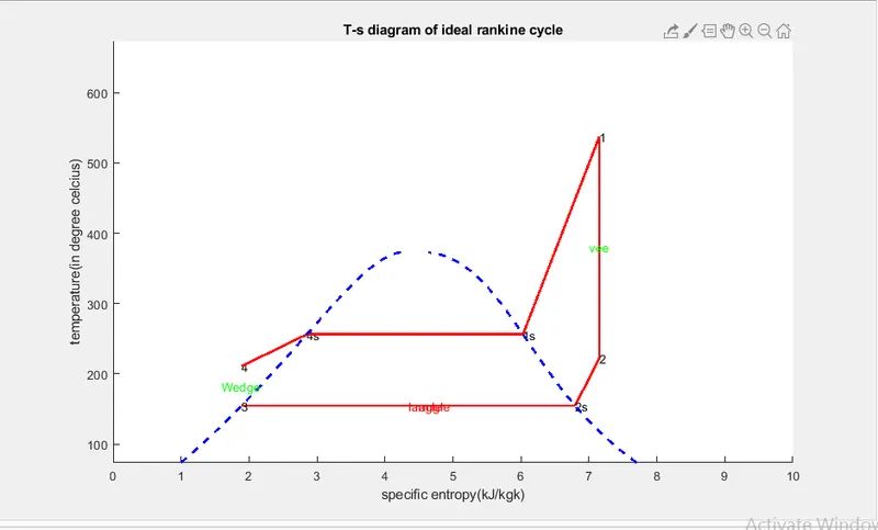
 figure(1) %T-s
 hold on
 grid on
 plot([S1,S2],[T1,T2],'r','linewidth',2)
 text(S1,T1,'1')
  text(S2,T2,'2')
  plot([S2,S2g],[T2,T2s],'r','linewidth',2)
  text(S2g,T2s,'2s')
  plot([S2g,S3],[T2s,T3],'r','linewidth',2)
 text(S3,T3,'3')
 plot([S3,S4],[T3,T3],'r','linewidth',2)
text(S4,T4,'4')
plot([S4,S1f],[T4,T1s],'r','linewidth',2)
text(S1f,T1s,'4s')
plot([S1f,S1g],[T1s,T1s],'r','linewidth',2)
text(S1g,T1s,'1s')
plot([S1g,S1],[T1s,T1],'r','linewidth',2)
plot(S_L,temp,'b','linestyle','--','linewidth',2)
 plot(S_V,temp,'b','linestyle','--','linewidth',2)
 %MARKING DIRECTION
 text(S1,(T1+T2)/2,'vee','HorizontalAlignment','center','color','g')
 text((S2g+S2f)/2,T3,'langle','color','r')
 text(S3,(T3+T4)/2,'Wedge','HorizontalAlignment','center','color','g')
    text((S1f+S1g)/2,T3,'rangle','color','r')
    title('T-s diagram of ideal rankine cycle')
    xlabel('specific entropy(kJ/kgk)')
    ylabel('temperature(in degree celcius)')


    % PLOT FOR H-s DIAGRAM
    figure(2)
    hold on
    grid on
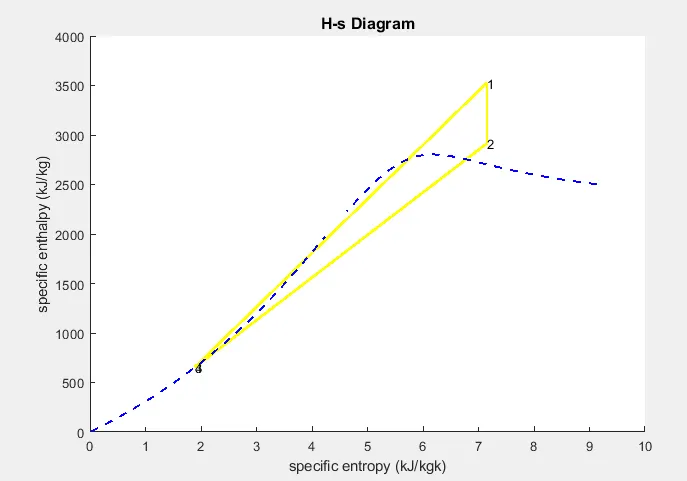
    plot([S1, S2],[H1,H2],'y','linewidth',2)
    text(S1,H1,'1')
     plot([S2, S3],[H2,H3],'y','linewidth',2)
      text(S2,H2,'2')
      plot([S3, S4],[H3,H4],'y','linewidth',2)
       text(S3,H3,'3')
       plot([S4, S1],[H4,H1],'y','linewidth',2)
     text(S4,H4,'4')

     plot(S_L,H_L,'b','linestyle','--','linewidth',1.5)
      plot(S_V,H_V,'b','linestyle','--','linewidth',1.5)

      title('H-s Diagram','Fontsize',12)
      xlabel('specific entropy (kJ/kgk)')
      ylabel('specific enthalpy (kJ/kg)')
- First of all, fprintf command is used to print the statements in the command window and also \n is used to move to the new line.
- Further , input command is used to feed the available variables for different values.
- Next , values of cp and cv are extracted from the xsteam for liquids as well as vapors.
- further entropy, enthalpy and temperature parameters at high and low pressures are extracted from the xsteam.
- Then , four state points are defined in the matlab and formulas are put down to calculate work done, efficiency as well as specific steam consumption.
-Finally, plotting is done when in the command window inputs values are entered.
RESULTS-
PLOT for T-s diagram;-
Plot for h-s diagram:-